Executables and Processes
Contents
14. Executables and Processes#
In this chapter we will explore what “native” binary programs are and begin our journey to learning how to create them though assembly programming.
This chapter follows two approaches to this material. In the first part we take an self-guided discovery approach. Here we use our knowledge and access to UNIX to follow our noses and poke around an executable to see what we can learn. In the second part of the chapter we take a more traditional textbook approach and present the conceptual model for how executables and processes relate to each other.
The following chapter includes several manual page entries. A reader is not expected to read these completely. They are mainly hear to illustrate how we can learn about the detail and document the precise way we can look them up later when we need too. In general you should skip the first few paragraphs. If there details that you should pickup on now the text will point you to them
14.1. “Running” Executables#
Perhaps the most basic thing we do on a computer is run programs. As we have seen, on UNIX, one of the main purposes of the shell is to let us start and manage running programs – Processes. As a recap remember that when we type a command like ls into a shell, it is not a built-in command. The shell will look to see if a file, with a matching name, exists in the list of directories specified by the PATH environment variable. If one is found (eg /bin/ls), and it’s meta data marks it as “executable”, the shell process will make calls to the UNIX kernel to create a new child process and try and “run” the file within the new process.
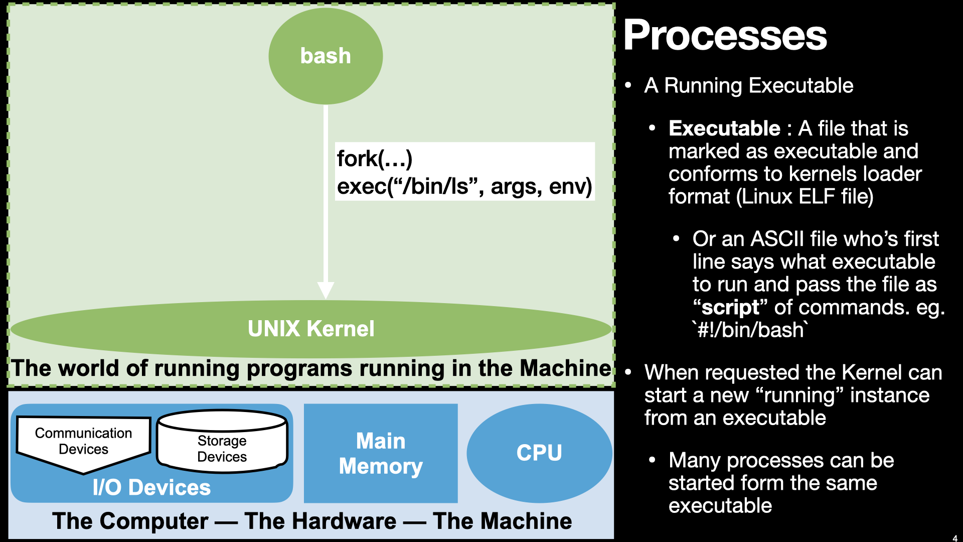
A: Bash calls kernel functions.
|
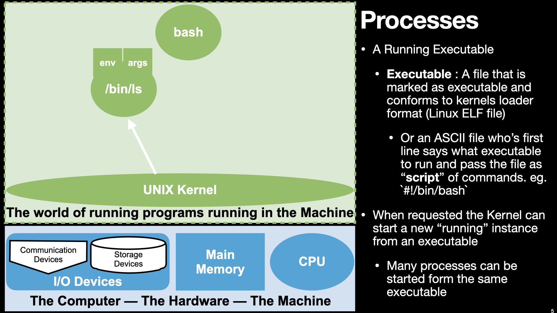
B: Kernel runs the program in new process.
|
As the figures state, there are two basic kinds of files that the kernel knows how to “execute” within a process. One is an ASCII file that has a special string at its beginning – #!<path of interpreter> and the other is an executable. The former is just a convenient way to allow programs like the shell to automatically be started with the contents of the file passed to it as a script to interpret. This makes it easy to write “scripts” that behave as if they where programs of their own. When in reality they are being interpreted as commands to the “real” program specified on the first line of the file. But the question, of course, is what exactly are real programs or executables.
14.2. What’s inside an executable#
Lets explore the /bin/ls file using our UNIX skills to see what we can figure out.
14.2.1. What does ls tell us about ls ;-)#
Running using ls to list the meta data of the file /bin/ls we see that it contains a sizable number of bytes. We also see that the permissions clearly mark it as being executable by all users of the system -rwxr-x-rx (if you don’t remember how to read this output see man ls).
14.2.2. Can we display its contents to the Terminal with cat?#
We encourage you to open a terminal and give this a shot. What happened? Well remember that all bytes that are sent to terminal are interpreted by the terminal as ASCII encoded information. It should be quickly apparent to you that whatever /bin/ls is it is NOT predominantly ASCII encoded information! Rather the bytes in it must be of some other kind of binary representation.
Below we pass the -v flag to cat so that it converts the non-ASCII values (things the terminal will not be able to print) in /bin/ls into a sequence of printable characters that represent their value, Specifically it using ‘^’ and ‘M-’ as prefixes followed by another character. You can see the man page of cat and the ASCII Table for more information.
14.2.3. Lets look at the byte values of /bin/ls using xxd#
So while the data in /bin/ls does not seem to be encoded in ASCII we can use other UNIX tools to translate the individual bytes of the file into a numeric ASCII value so that we can at least see what the values of the bytes of the file are. There are several such tools we could use. Examples include: od (octal dump), hexdump, and xxd. We will use xxd
xxd conveniently lets us look at the value of a file represented in base 2 binary digits or base 16 hexadecimal digits. We will use the following command to display the first 256 bytes of the file in binary: xxd -l 256 -g 1 -c 8 -b /bin/ls
Where:
-l 256is used to restrict ourselves to the first 80 bytes-g 1is used to tell xxd to work on units/groups of single bytes-c 8is used to print 8 units/groups per line-bmeans display the values in base 2 (binary) notation
This causes xxd to open /bin/ls and read the first 256 bytes. It examines the value of each byte read and translates it so that it produces a string of eight ASCII characters of either 0 or 1 depending on the value of the bits of the byte. In this way we can use xxd to display the byte values of a file. The left hand column of the output encodes the byte position in the file that the line of data corresponds too. These position values start at zero are in hexadecimal notation (eg. 00000010 is 16 in decimal). On the far right of each line xxd prints an ASCII interpretation for any byte values that correspond to printable ASCII characters (otherwise it prints a .).
Using hexadecimal notation we get more concise visual representation
So while it might look cool, without knowing how to interpret the byte values it really does not provide us much insight as to what makes this file a program that lists the contents of directories.
14.2.4. Using the UNIX file command on /bin/ls#
While there are no explicit file types in UNIX that tell use what kind of information is in a file (we are expected to know) there is a command that is very good at examining a file and guessing what kind of information is encoded in the file based on a large database of test. This command is called file. Here is its manual page.
Well let’s see what file has to say about /bin/ls.
Ok cool! File tells us /bin/ls is an ELF file. You might have noticed that the xxd output showed the ASCII characters ELF near the beginning of the file. This is due to the fact that this is part of the ELF standard format to make recognition of them easier.
14.2.5. ELF Files - Executable and Linking Format Files#
So what exactly is an ELF file? Lets see what the manuals have to say. P.S. You are not expected to understand what it is saying at this point.
Wow, that’s a lot of information that does not make much sense at this point. However, it is nice to see that it seems to be a format for encoding “executable” files ;-)
Now, as it turns out, there several tools such as readelf and objdump that are designed to decode elf files. But it is not clear that this is going to help much until we get a better conceptual understanding of what it means to encode a program for execution in a process.
For your interest here is the output for readelf --all /bin/ls and objdump --all /bin/ls which dump summary information about the /bin/ls executable.
As a teaser here is some actual “content” that objdump can extract and decode from /bin/ls. Specifically this command, objdump -d /bin/ls ‘disassembles’ the binary.
14.3. Executing an Executable in a Process#
Lets try this from the other direction. We know that there is a call to the OS to run an executable. Lets see what we can find out by examining the OS documentation.
Lets start by looking up the manpage for the operating system call exec. At this point we are going to ignore the programming syntax and mechanics and rather focus on what we can learn in broad strokes from the manual page.

Notice in the above output we see line numbers for the man page. The
mancommand itself does not support line numbers but thecatprogram does if you pass it the-nflag. So instead of just using the commandman execon its own we have sent its output tocat -nusing the pipe syntax of the shell:|. So our combined shell command is:man exec | cat -n. Remember ot notice these things as UNIX can teach many good programming habits like the value of breaking our software down into small reusable parts and having a standard way for combining those parts (eg a pipe).
We want to focus on the first two paragraphs of the description (lines 27 - 33). These sentences imply that running a program loads a new “process image” over the current one. Remember, in the Introduction we used the term memory image. It is not a random coincidence that we are seeing the same terminology here. Further reading between the lines, the “file” to be executed contains or is the base of the new process image. Given that this man page tells us that exec is really just a front end of execve, lets look at that man page and see if we can learn a little more.
Let’s focus on lines 13-21 and 41-43. Again, we see that the wording is all about replacing the contents of an existing process with the value from the executable file. Further, we that some parts of the new process will be newly initialized: stack, heap and data segments. In lines 41-43 we are told that execve, assuming success, will overwrite certain parts of the text, data and stack of the process with the contents of the executable file (newly loaded program). So, vaguely, we are starting to get the picture that an executable encodes values that get “loaded” into a process to initialize the execution of the program contained within it.
Our task now is to start putting the pieces together. We need to get a better idea of processes are, their relationship to binary executable files and how we go about encoding a program into an executable.
14.4. Binary Executables as Process Images.#

|
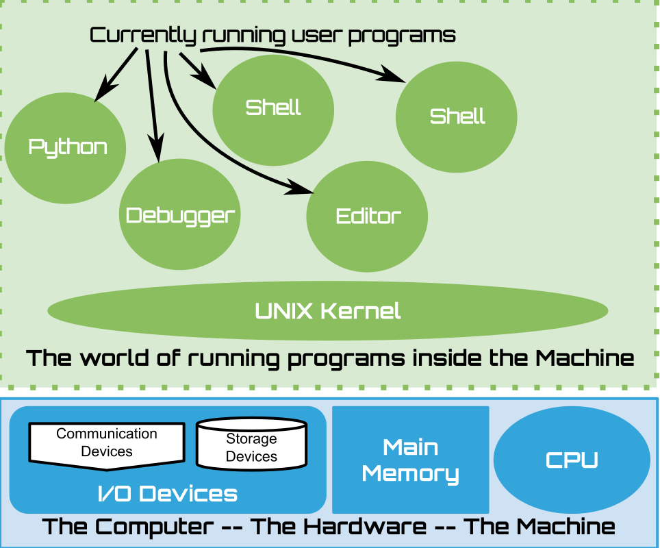
Given our basic view of how a von Neumann computer operates we can see that what we load into memory drives the CPU’s execution. But how does this relate to the what is going on when we are running an operating system like UNIX which constructs a world of running software down into an OS kernel and a set of user processes?
|
From our perspective, as users of an operating system, we navigate the file system to find programs, in the form of executable files, to launch. In UNIX we use a shell like bash to do this. Bash on our behalf calls down into the UNIX Kernel requesting that it creates a new process from the specified executable file. In UNIX bash does this with two UNIX kernel system calls (fork and exec).
|
|
|
14.4.1. Process Contexts#
To better understanding of how processes, executables and the von Neumann model of execution relate, we need to dig down a little further.
|
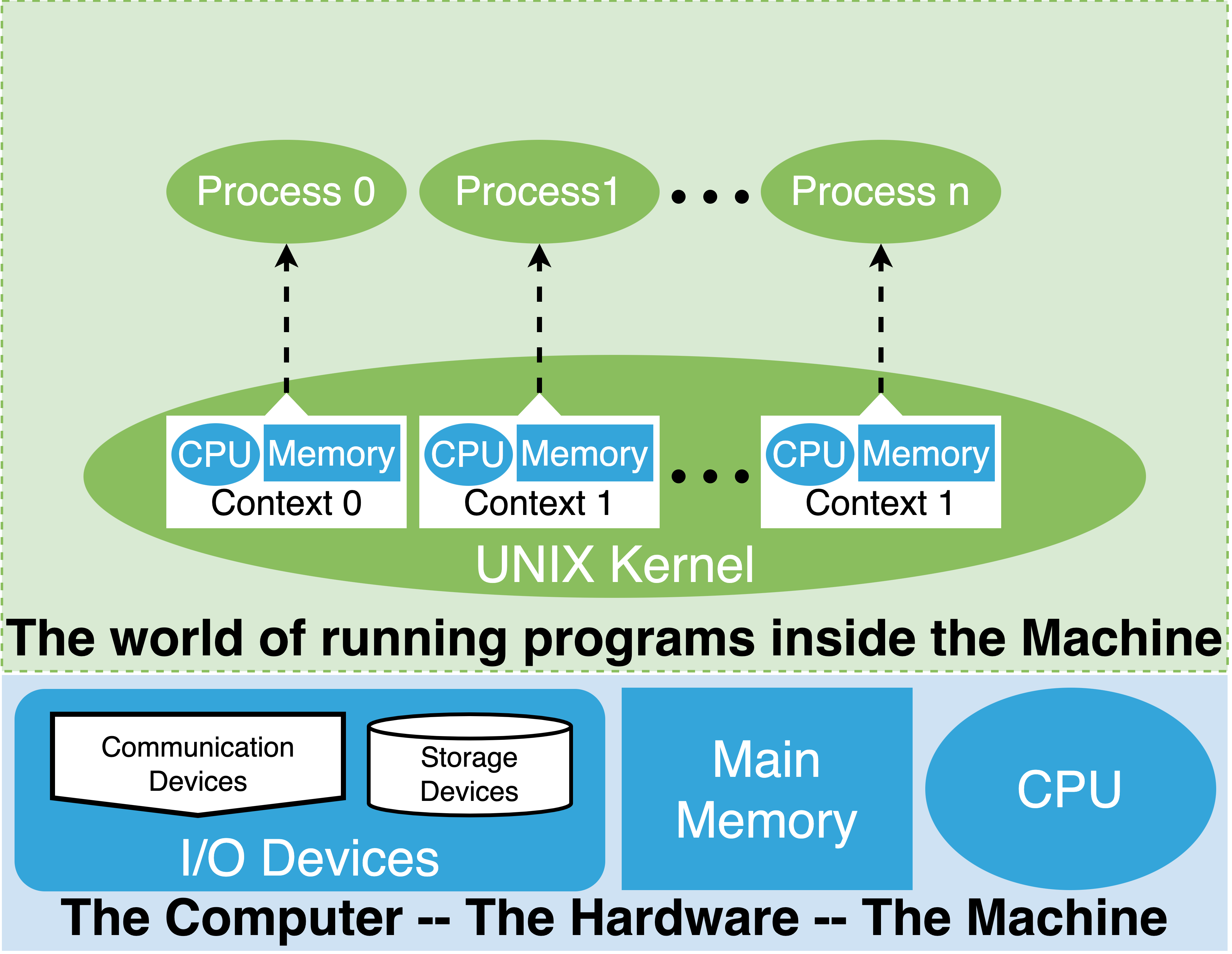
Each time we ask the OS kernel to launch a binary executable, the kernel creates a new process “Context”. Each context is a collection of data structures that the kernel uses to represent the memory for the process and the CPU registers. A process is like a restricted virtual von Neumann computer.
14.4.1.1. Context Switch – Scheduling Processes#
Using the privileged execution features of the hardware the kernel “switches”, the contents on and off the real CPU and memory of the computer.
To let a particular process execute, the kernel loads the GPRS of the CPU from the context and sets SPRS of the CPU so that all “normal” mode memory accesses are directed to the process context’s memory data structures. Once these steps are done, the kernel resumes “normal” execution via a privileged instruction and the particular process will execute on the CPU in context of its own memory.
When the kernel wants to switch which process is executing, it takes over the CPU, saves the values of the GPRS into the process context of the current process, and then follows the steps above to set a different context as the currently executing one.
The act of picking which process to execute on the CPU and switching between them is called scheduling and is a core function of the operating system. Processes are what lets us treat our computers like many little sub-computers, each which can execute based on an independent view of the CPU and memory. While it is executing, the process has control of the CPU and can conduct memory transactions.
From the perspective of the von Neumann architecture, the thing that the process is missing is the ability to conduct I/O. This is on purpose to avoid the programs that run in processes needing to deal with the The Ugly Underbelly of I/O devices. Rather, as we will see in other chapters to conduct I/O processes it makes requests to the kernel to control the I/O devices on it’s behalf. The OS kernel hides the details of I/O from the process and ensures that I/O is carefully arbitrated between the multiple running processes. In UNIX the core abstract primitive for I/O it provides processes are functions for creating, writing and reading files.
The exact details of how processes, contexts and scheduling are implemented vary between operating systems and the details of the hardware. The level of detail we have covered is enough for us to continue our exploration of how processes and executables are related.
14.4.2. Executables: Initial Images for creating Process Contexts#
We can now put things together. In the section above we discussed how the Kernel represents processes with context data structures and uses them to schedule the CPU across processes. But where do the initial contents of memory for a process come from?
This is the primary role that binary executables files serve. Binaries are files that describe the initial memory contents for a process; the exact values that the process contexts data structures should be initialized with and their addresses. From this perspective, an executable is the initial memory “image” that the OS “loads” into a newly created process context. The reason we call it an image is that it is precise map that describes what the memory of a process should initially look like. While the process executes the memory context will change and evolve diverging from the initial image of the executable.
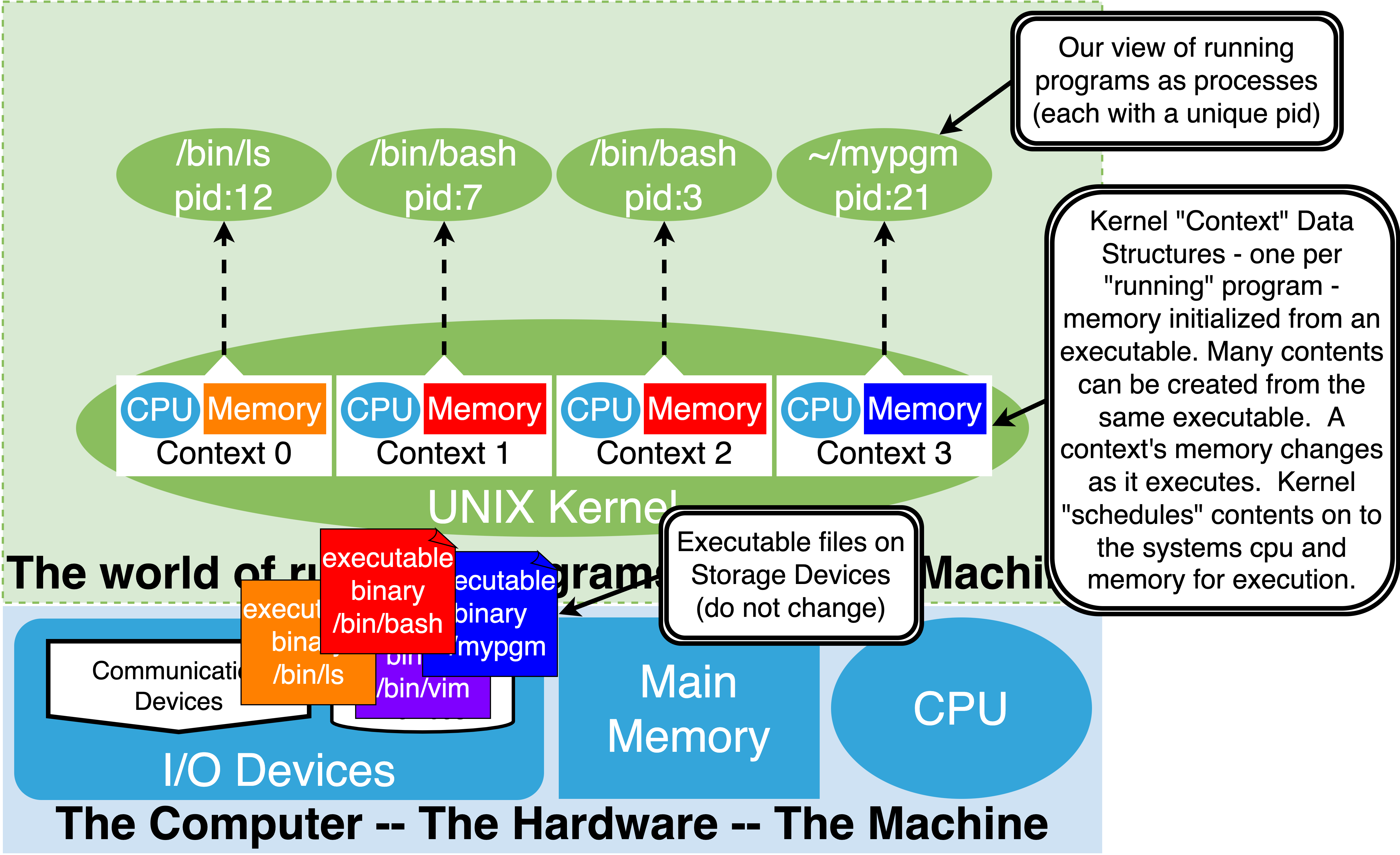
The figure below illustrates this relationship with a simple example.
|
At the bottom of the figure, four executable files are illustrated as colored document icons; 1) /bin/ls (orange), 2) /bin/bash, 3) mypgm (blue) and 4) /bin/vim (purple). These files are located on the storage I/O devices. The rest of the diagram illustrates a UNIX kernel that is running four processes. With the kernel, four contexts are shown, one for each process. The memory of each context is colored with the color of the executable they were started with. In this case Context 0 was initialized with /bin/ls, Context 1 and Context 2 from /bin/bash and finally Context 3 with an executable file called mypgm. Above the kernel is the abstract view of the running processes that correspond to the contexts. The kernel assigns each process a unique identifying number called a Process Identifier (pid).
In UNIX the ps command lets us explore this view of the systems, listing the running process. ps can display many attributes of the processes including the pid and the executable it was initialized with.
Executables are used to initialize the memory for new process contents. Many contents can be created from a single executable. Each process, after it is created, is an independent running instance of the executable. In the figure, we can see that two processes have been started from the bash executable. As the processes execute, they modify their memory contexts but the original executable is not modified and is preserved as a starting point for any new contexts started from it. This is how we can have many independent “shell” processes running all spawned from the same binary. Note that while many independent processes can be running at a given time, started from one or more executables, there is always only one OS kernel running that manages these processes.
Once initialized the process contents are scheduled by the OS onto the CPU and memory, as described in the prior section, and continue executing until they terminate.
So now that we know how executables relate to processes, what remains is learning how to create executables. Then we will be able to start processes from images that we constructed. Once we understand this then the goal will be learning how to prepare the contents of an executable so that it encodes our programs!
Two of the techniques used are: 1) Dynamic loading and linking and 2) Memory Paging.
Rather than having every executable contain an exact copy of it’s initial memory image, dynamic loading and linking allows the executable to only contain the parts of memory that are unique to the program. Any common libraries of routines an executable uses are not in the executable. Rather the executable simply includes a list of the libraries and routines it requires. When creating a process for such a “dynamically linked” executable a dynamic loader-linker will validate that the required files can be found. It then ensures that as the process is run the values from the other file are added to the process context. This approach has several nice properties. The sizes of binaries are considerably smaller and it now possible to upgrade libraries and have new process, started from exiting binaries, automatically use them.
The second technique, Memory Paging, refers to the OS using the Memory Management Unit facilities of the CPU to avoid having the entire memory of a process context present in the computers physical memory. Specifically, the OS uses hardware “paging” features to carve up a process context memory into chunks called pages. At any given time the only pages that need to be present are the ones that the executing process is currently conducting memory transactions too. The other pages, of currently schedule process and, non-schedule processes can be stored on I/O devices. The OS then shuffles the pages in and out of main memory as needed. Treating the main memory as a form a “cache” for the active pages of the running processes. This allows us to run many programs who’s “virtual” memory is larger than the physical memory of the computer.
Virtual Machines are an advanced scheme that uses CPU support to partition the computer so that multiple independent OS Kernels can be started. Each believing it is running directly on the hardware and starting and managing it’s own processes.
14.5. Creating executables#
Given the nature of von Neumann execution and what we know now, “Programming” a process means preparing an initial memory image in the form of an executable.
To do this we will use the two tools that are the foundation for constructing executables: an assembler and a linker.
While many high level programming languages exist in the end to get something to execute it must be represent as binary values in memory. An assembler and linker are the base tools that provide programmers the to directly specifying what the contents of an executable should be.
The rest of this chapter focuses on introducing these tools and how to practically use them to create an executable. We will, however, defer our discussion of how to encode useful programs within executable to later chapters. Rather, we will culminate this chapter with the ability to create an empty executable that will let us create a “blank” process. While this process will not be useful on its own we will be able to use it with a debugger to directly explore the internals of the CPU and memory of a process and learn how to use the debugger as more than a debugger.
14.5.1. Assemblers#
The assembler is a program that processes commands in a file that directs it to create fragments of memory contents. The linker, discussed next, will combine these fragments according to a generic layout to create an executable.
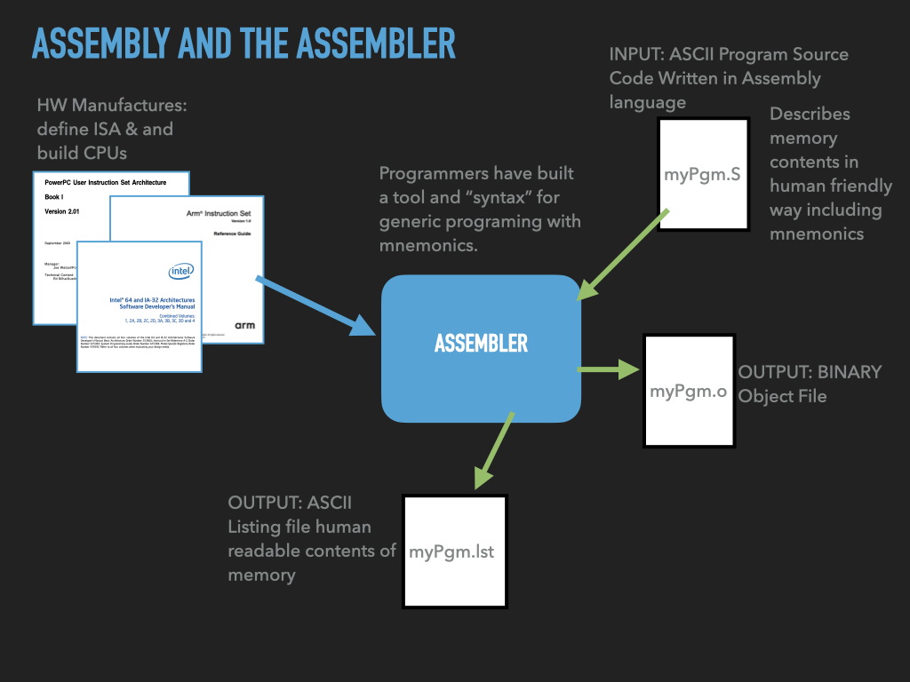
The code we write in the syntax of the assembler is assembly code and is a combination of CPU specific mnemonics and special assembler specific directives . We write assembly code files in ASCII with an ASCII editor. Traditionally on UNIX systems we use the suffix .s or .S for assembly code files.
|
As illustrated in the figure authors of the assembler use the CPU manufactures documentation to write the assembler. The assembler is written to be able to translate the CPU mnemonics, written in ASCII into the CPU specific binary values that encode the specified instruction.
The assembler directives allow us to write arbitrary values that should be placed in memory. The assembler understands various formats (such as hex, binary, signed and unsigned integers, ASCII, etc) and sizes. The assembler will convert the values we write, in the various formats, into the correct raw binary values that should be place in memory. Directives also let us control both the relative and absolute placement of values.
In addition to mnemonics and directives, assemblers allow a programmer to introduce symbolic human readable labels for the addresses of particular values. The symbolic labels, or simply symbols, allow us within our assembly code to refer to the values at the location of the symbol. It will be the linker’s job to both set the address for a label and replace the reference to the symbols address to the address it assigns to the symbol.
Finally and by no means least the assembler allows us to provide comments that explain what our code is doing. It is particularly important to carefully document assembly code given its cryptic nature. It is not uncommon for the comments in an assembly file to far out number the actual code lines.
Assuming that there is no errors in the assembly code, the assembler will translate our input file into what is called an object file. This file, in general, will encode a sequence of values for both the text and data of our program, however, the exact locations will not be specified. In addition to the values the file can encode various descriptive facts so that the linker can connect up our code with code generated from other object files. It can also contain information that can be saved in the final binary that other tools like the OS and debugger can use to understand what the bytes of the executable mean. For example, it can contain debugger information that will allow the debugger to know what source code file and how the lines within it correspond to particular opcode bytes in memory.
Traditionally assemblers can produce a “listing” file which is an ASCII document that describes the actions and output that the assembler took and produced while processing the input assembly source file. The listing file can be very useful in understanding how you code we translate into byte values and what symbols it introduces and those that it references.
As we progress we will understand more of the features and details of the assembler and its syntax through examples. For the moment we are only concerned with a general understanding of it role and how.
14.5.1.1. GNU Assembler (gas)#
The particular assembler that we will be using is the GNU Assembler (gas). As stated before we will learn its basic syntax as we work through various examples.
When we use gas to process INTEL mnemonics we will be using the mnemonic syntax that is compatible with the INTEL manuals. There is another standard that was introduce by AT&T, for writing INTEL mnemonics but was will avoid this syntax.
The following is the manual for gas. Section 3.5 describes statements which can be very helpful in learning to read and write gas assembly.
14.5.2. Linkers#
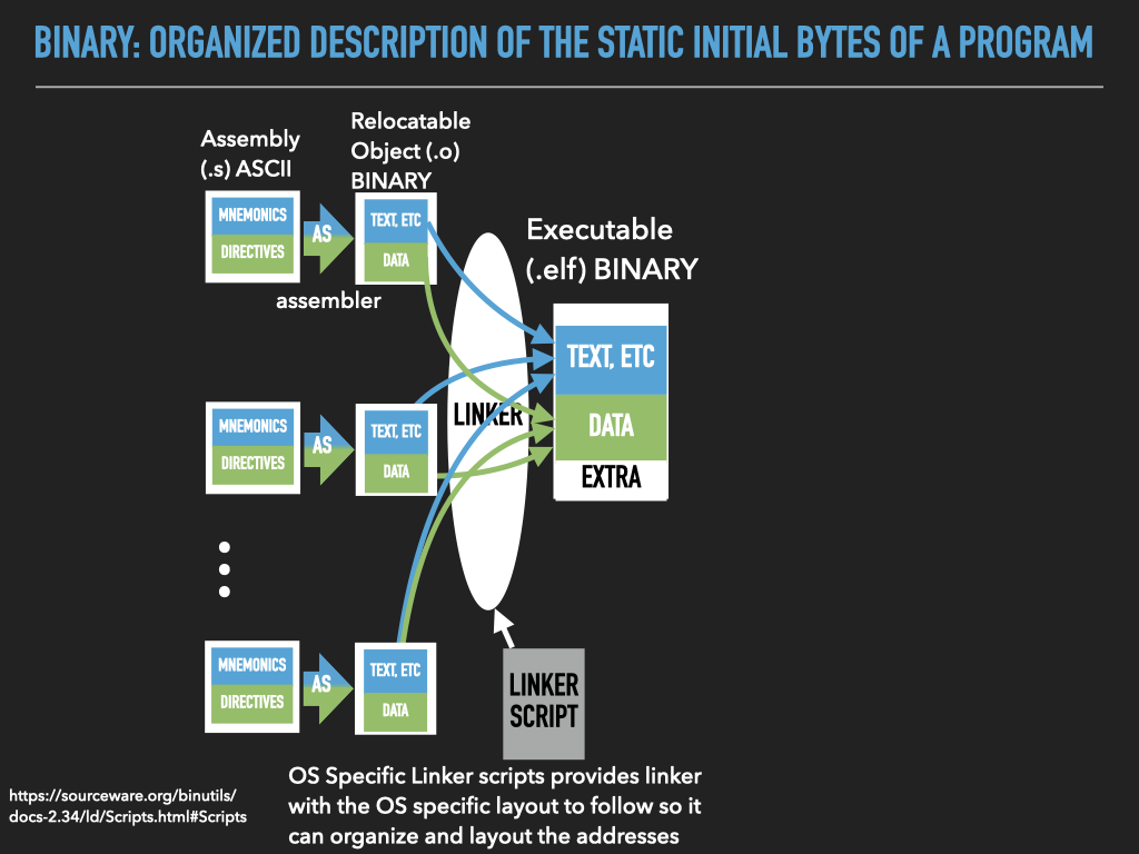
The process of constructing executables has purposefully been broken down into two steps to make it easier to construct programs out of a collection of code. Specifically as we read above an assembler produces fragments of memory values called object files.
The basic idea is that programmers write various reusable chucks of assembly code that introduce data and text stored in object files. The data and text from multiple object files can then be combined to produce a final executable by a linker. Where the linker takes object files, libraries of object files and a generic description of how the text and data should be laid out, located in memory, to be compatible with the OS process model.
|
While this approach might seem unnecessarily complicated at first it make our lives as programmers much easier. First it provides us with the ability to compose our programs out of our own libraries of code and code provided by others. Secondly we don’t have to worry about where exactly everything ends up in memory. Rather the linker will be given all the inputs including general directives for how to layout the text and data of an executable for it to be compatible with a particular OS. With all of these this as input it will organize the values of our code into a coherent image that has the text and data correctly laid out and all symbols and their references will be carefully connect.
The operation of the linker may seem quite vague at this point. In later chapters we will fill in the details when we discuss how memory gets assigned by the OS to a process context when “loading” an executable.
14.5.2.1. GNU Linker (ld)#
Like the assembler the specific linker we will be using is the default linker used by the Linux Operating system, the GNU Linker (ld). The following is the manual for ld.
14.5.3. Creating and using our first executable.#
Our goal now is to put all the pieces of this chapter together to create our first executable. While it will be a valid executable that the OS can load, it will only contain a small number of bytes that will all be zero. As such when we go to run it we don’t expect it to behave in a particularly useful way.
However, we will be able to use it with the debugger to explore the process that is created from the the binary. In some sense it is the simplest process we can create that has at least some initialized memory within it.
14.5.3.1. The source code#
CODE: Our very own 'empty' binary
/*  General antomy of a assembly program line
[lablel]:   <directive or opcode> [operands]  // comment
*/
	.intel_syntax noprefix        # assembler syntax to use <directive>
	                              # set assembly language format to intel

	.text                         # linker section <directive>
	                              # let the linker know that what follows are cpu instructions to
	                              # to be executed -- uposed to values that represent data.
	                              # For historical reasons cpu instructions are called "text"

	.global _start                # linker symbol type <directive>
	                              # makes the symbol _start in this case visible to the linker
	                              # The linker looks for an _start symbol so that it knows address
	                              # of the first instruction of our program

_start:                               # introduce a symbolic (human readable) label for "this" address
	                              # associates the address of this point in our program with the
	                              # name following the ':' -- in our case _start
	                              # In our program or in the debugger we can use this name to
	                              # to refer to this location -- address.  And thus the values
	                              # that end up here.
	.byte 0x00, 0x00, 0x00, 0x00  # .byte directive place value at successive locations in memory
	.byte 0x00, 0x00, 0x00, 0x00  # (https://sourceware.org/binutils/docs/as/Byte.html#Byte)
The above code is the contents of a file we have named empty.s. In reality it is not really empty but rather contains four bytes of zero.
This code has been extensively commented so that we can use it to learn a little about the assembly syntax and what it lets us do. In general, as said before, it is good practice to write lots of comments in your assembly code. The following is an un-commented version:
    .intel_syntax noprefix
    .text
    .global _start
_start:
    .byte 0x00, 0x00, 0x00, 0x00
    .byte 0x00, 0x00, 0x00, 0x00
As described the keywords that start with . are directives. The assembler does not attempt to interpret them as CPU mnemonics. Rather
they are various command that control how the assembler behaves.
Unsurprisingly, the first statement, .intel_syntax noprefix, tells the assembler
that we want to use the INTEL syntax for writing mnemonics. The next statement .text is a “section” directive, more verbosely it could have been written
.section .text. It tells the assembler to let the linker know that any values that follow belong with the text values of the final binary. If we want to put values in other sections, such as data we would then switch sections. The next line .global _start tells the assembler to place the symbolic label that is introduced on the following in the list of “external” symbols that this object file is making visible to the other object files. The reason we do this is due to a requirement that every executable needs to define a symbol that tells the OS how to initialize the PC when it creates a new process context from the executable. This symbol is call the entry point. On Linux the default symbol the linker looks for as the entry point is _start. So in combination the two lines say that file is defining an externally visible symbol _start and defines it to be the location of the values that follow. Since we have not inserted any values yet we are still at the beginning of the text memory that this object file defines.
The next two lines define raw hex byte sized values that we want to place into the memory object. The .byte directive expects us to list one more comma separated values that the assembler will translate into binary values and place in the object file. The assembler understands many formats for the values.
In our case we are using hex notation and simply specify eight bytes all zero valued. Each byte moves the insertion point to the next offset relative to the current section. As such these two lines tell the assembler that we want this object file to contribute 8 zero value bytes to the text values of the final linked executable.
14.5.3.2. Assembling the source into an object file#
The following invocation of the assembler will translate the empty.s into empty.o. The -g flag tells the assembler to keep information in the object file that the debugger can use. The -o empty tells the assembler what the name of the output object file it should create.
Using ls we see that indeed the assembler created a file called empty.o. Note it is quite a bit bigger than the 8 bytes that we want loaded into memory. That is because there is lots of extra information that must be put into an object file so that link knows how to work with it.
14.5.3.3. Linking the object file into an executable#
While we only have one object file that composes our binary we will need to have the linker process the object file and convert it into a executable object file. The ld has built into a file called the link script that describes where thinks, like the text and data of the executable files need to go to be compatible with the OS, Linux in our case. This includes encoding the address where the _start symbol gets place as the entry point for the binary.
The following is the command to link our single object file into an executable. Again note that we pass ld -g flag also telling it to generate and keep information for the debugger in the executable.
Using ls again we see that the linker produced the executable empty as directed by the -o empty argument.
Notice this time it does have the execute permissions set.
14.5.3.4. Running the executable#
Ok lets run it.
14.5.3.5. Segmentation Fault#
The message Segmentation fault indicates that the kernel informed the shell that the kernel terminated the process that it started to run the empty executable. Specifically the kernel told the shell that empty did an “Invalid memory reference” and so the kernel terminated the process. An invalid memory reference means that the process trying to do a memory transaction to an address that did not have valid memory associated with it.
In later chapters we will discuss why memory is invalid an how to create valid memory. For the moment it suffices to say that an memory that our process will have needed to be defined by the executable. An in our case we only created 8 bytes of memory we knew was valid.
The real use of the empty binary is that it allows us to create a very simple process that we can use the debugger with.
14.5.3.6. Using empty with gdb#
In the following session we use gdb to create a process and then explore, modify and execute an instruction within it. Other chapters will go into the details this is just to give us a flavor of how we can use gdb to explore the relationships between an executable and a process created from it.
The following is an explanation for what is was done
set the disassembly syntax of gdb to intel
set disassembly-flavor intel
open the empty assembly file
file empty
We can now printf explore the values within the executable This includes finding out where a symbol got located including our entry point
p /x &_start
Before we start a process we want to have gdb freeze it before any instructions within it execute. So we set a break point at the address of the entry point.
b &_start
Ok let’s start a process from the open executable
run
At this point the a process has been created but it is frozen at the breakpoint and we can control it from gdb. We can print information about it
info procWe can look at it’s registers
info registersWe can work with individual registers
p /x $raxp /t $raxp /d $raxp /x $rip
We can examine memory
x/8xb 0x401000
We can even ask gdb to disassemble memory
x/2i &_start
We can also write new values into memory. Lets uses this this ability to replace some of our zeros with the values that encode an instruction :
popcnt rbx, rax. Each time we add a new value we will ask gdb to display the memory and to disassemble what it finds there so we can see our progress.set {unsigned char}&_start = 0xF3x/5xb &_startx/1i &_startset {unsigned char}(&_start+1) = 0x48x/5xb &_startx/1i &_startset {unsigned char}(&_start+2) = 0x0Fx/5xb &_startx/1i &_startset {unsigned char}(&_start+3) = 0xB8x/5xb &_startx/1i &_startset {unsigned char}(&_start+4) = 0xD8x/5xb &_startx/1i &_start
Cool those five bytes to encode the instruction we want. Lets display those bytes in various other forms
In binary notation:
x/5tb _startAs signed decimal numbers:
x/5db _startAs unsigned decimal numbers:
x/5ub _start
Lets display the current contents of the two register that our instruction uses an operands
p/x {$rax, $rbx}
Before we execute the instruction lets remove the break point to make our life easier
delete15 We can use gdb to execute one instruction at a timestepi
Lets look to see if the registers have changed
p/x {$rax, $rbx}
Lets try again but lets put a value in rax
set $rax = 0b1011
Again we print the value of the registers to be sure we know what values are in them before we execute the instruction
p/x {$rax, $rbx}
Remember the pc tells us where the next instruction is
p /x $pc
So we need to reset it back to the address we placed the instruction which was the address of
_startset $pc = $_startstepip/x {$rax, $rbx}
Cool rbx now has the number of bits set to one that the value in rax has – its “population count”
14.5.4. The code to create an executable for a larger empty process#
The following code replaces the two lines of .byte directives with a single .fill directive that inserts in this case 256 zero valued bytes into memory at _start
CODE: An empty binary with a little more room.
0: 	.intel_syntax noprefix        # syntax directive
1: 	.text                         # linker section <directive>
2:
3: 	.global _start                # export symbol _start to linker
4: _start:                           # start symbol
5: 	.fill 256, 1, 0x00            # https://sourceware.org/binutils/docs/as/Fill.html