17. Representing information - Preliminaries: Bits, Bytes and Notation

In general most physical components of a computer store, transmit, or operate on a pattern of binary values. The pattern is a fixed size collection of bi-stable physical units. Bi-stable means that each unit within the collection can reliably be in one of two distinct states. Depending on the device, various different physical mechanisms can be used to represent the values. Some devices, such as older hard drives, use magnetic polarity — north vs south magnetic force. In these devices a surface is coated with a magnetic material. By dividing the surface into non-overlapping regions, we form units that individually and independently can have their magnetic polarity changed and detected. Integrated into these devices is one or more electro-magnetic heads that can “write” or “read” a region, when the region is below them. Writing means setting the regions polarity to north or south and reading means detecting the regions current polarity. The head is an electrical device. When reading, it generates either a high or low voltage on a wire depending on the polarity of the region. Similarly an electrical signal can be used to direct it to set the polarity if desired.

Modern Solid State Drives (SSDs) and things like “USB sticks” contain electrical cells that serve as their units. No head is required for these devices as the cells can be directly accessed. Depending on the technology used, the cells might represent states using electrical charge or changes in their electrical resistance.

Other devices such as memory “chips” use cells that actively consume electricity to maintain their values. If electricity is lost, eg your battery dies, then their values are lost. However, unlike Hard drives, SSDs, and USB sticks, devices composed of these chips can be written and read very fast using electrical voltages on wires that are directly connected to them. These components are often called the Memory or RAM (Random Access Memory) of our computers. The CPUs have direct electrical connectivity to RAM which serve as the working memory for the active programs running on our computers.

From our perspective, the key point is that regardless of the technology, storage devices can be abstractly thought of as a fixed size array of units that can take on one of two distinct states. Further the devices can be controlled and accessed through electrical signals.

This last part is important as the majority of high speed devices, like RAM and CPUs, used in a computer use electricity (or in some cases light). High vs low electrical voltage is in some sense the universal language for binary values in a computer. Circuits within the CPU operate on electrical voltages to implement functions on the patterns of high and low values. Collections of wires, called buses, interconnect components of the computer and allow them to transmit patterns between each other in controlled and orderly ways. Like most things, the transfers are initiated and controlled via the the instructions of our programs, executed by the CPU. For example the following Intel instruction sequence directs the components of the computer to transmit 64 binary values from one location in RAM to another via a register in the CPU.

mov rax, qword ptr [4208]
mov qword ptr [4216], rax

Even our I/O device, such a touch screen, is really just a device in which electrical charges can be used to control the individual picture element (pixels). Pixels are controlled by turning on or off specific light emitting components or translating pressure on the screen into electrical signals on wires for the particular location touched.

While the physical part of the computers can store (eg RAM), transmit (eg Busses) and operate on (eg CPUs) binary patterns via electrical voltages, they do not enforce a particular “meaning” on the patterns. In some sense the components of the computer form a blank sheet of “paper” which a programmer can use to represent and manipulate information using patterns of electrical signals and the capabilities of the CPU, memory and I/O devices.

17.1. Bits and Bytes

Given that the components of a computer are built to work with discrete binary, two valued, patterns, it is natural for us to use arrays of binary digits (bits) to represent what values we want the components to store, or the operations we want done.

As such, the world of software is really a world in which we translate our ideas into arrays of bits. Remember, however, as we continue our discussion of information representation that the components of the computer are simply working on patterns of electrical signals, charges, resistance, magnetic polarity, etc. They do not store or operate explicitly on strings, integers, floats, functions, instructions, hexadecimal values or even ones and zeros. All these notions are how we as programmers use the values within the components to represent information (including the instructions of our programs that implement algorithms).

17.1.1. The Byte

Fig: A byte as 8 switches: We can visualize a byte as an array of 8 bits. As a programmer we think of a computer as many such arrays. Each byte has some particular location in the computer and a particular value that it current stores. The value can be thought of as the current configuration of its switches: on or off.

The standard unit that we have settled on is a pattern of 8 bits, binary digits, called a byte. Sometimes we break a byte down into two 4-bit quantities called a nibble. Bytes are also often grouped into larger units. However, the names for these larger units are unfortunately not always consistent. Some conventions, such as those used Intel products, call an array of two bytes a word, four bytes a double word and 8 bytes a quad word. However other conventions refer to four-byte arrays as a word, a two-byte arrays as half word and an 8-byte array as a double word. Given this ambiguity it is often best to use bit lengths such as 8, 16, 32, 64, 128, 256 to avoid confusion. Nonetheless, sometimes we do not have a choice but to be aware of the convention that is in use to understand what is meant by the code or manual we are reading.

Table of all 2⁸ = 256 possible binary byte values.

[b7	b6	b5	b4	b3	b2	b1	b0]
0	0	0	0	0	0	0	0
0	0	0	0	0	0	0	1
0	0	0	0	0	0	1	0
0	0	0	0	0	0	1	1
0	0	0	0	0	1	0	0
0	0	0	0	0	1	0	1
0	0	0	0	0	1	1	0
0	0	0	0	0	1	1	1
0	0	0	0	1	0	0	0
0	0	0	0	1	0	0	1
0	0	0	0	1	0	1	0
0	0	0	0	1	0	1	1
0	0	0	0	1	1	0	0
0	0	0	0	1	1	0	1
0	0	0	0	1	1	1	0
0	0	0	0	1	1	1	1
0	0	0	1	0	0	0	0
0	0	0	1	0	0	0	1
0	0	0	1	0	0	1	0
0	0	0	1	0	0	1	1
0	0	0	1	0	1	0	0
0	0	0	1	0	1	0	1
0	0	0	1	0	1	1	0
0	0	0	1	0	1	1	1
0	0	0	1	1	0	0	0
0	0	0	1	1	0	0	1
0	0	0	1	1	0	1	0
0	0	0	1	1	0	1	1
0	0	0	1	1	1	0	0
0	0	0	1	1	1	0	1
0	0	0	1	1	1	1	0
0	0	0	1	1	1	1	1
0	0	1	0	0	0	0	0
0	0	1	0	0	0	0	1
0	0	1	0	0	0	1	0
0	0	1	0	0	0	1	1
0	0	1	0	0	1	0	0
0	0	1	0	0	1	0	1
0	0	1	0	0	1	1	0
0	0	1	0	0	1	1	1
0	0	1	0	1	0	0	0
0	0	1	0	1	0	0	1
0	0	1	0	1	0	1	0
0	0	1	0	1	0	1	1
0	0	1	0	1	1	0	0
0	0	1	0	1	1	0	1
0	0	1	0	1	1	1	0
0	0	1	0	1	1	1	1
0	0	1	1	0	0	0	0
0	0	1	1	0	0	0	1
0	0	1	1	0	0	1	0
0	0	1	1	0	0	1	1
0	0	1	1	0	1	0	0
0	0	1	1	0	1	0	1
0	0	1	1	0	1	1	0
0	0	1	1	0	1	1	1
0	0	1	1	1	0	0	0
0	0	1	1	1	0	0	1
0	0	1	1	1	0	1	0
0	0	1	1	1	0	1	1
0	0	1	1	1	1	0	0
0	0	1	1	1	1	0	1
0	0	1	1	1	1	1	0
0	0	1	1	1	1	1	1
0	1	0	0	0	0	0	0
0	1	0	0	0	0	0	1
0	1	0	0	0	0	1	0
0	1	0	0	0	0	1	1
0	1	0	0	0	1	0	0
0	1	0	0	0	1	0	1
0	1	0	0	0	1	1	0
0	1	0	0	0	1	1	1
0	1	0	0	1	0	0	0
0	1	0	0	1	0	0	1
0	1	0	0	1	0	1	0
0	1	0	0	1	0	1	1
0	1	0	0	1	1	0	0
0	1	0	0	1	1	0	1
0	1	0	0	1	1	1	0
0	1	0	0	1	1	1	1
0	1	0	1	0	0	0	0
0	1	0	1	0	0	0	1
0	1	0	1	0	0	1	0
0	1	0	1	0	0	1	1
0	1	0	1	0	1	0	0
0	1	0	1	0	1	0	1
0	1	0	1	0	1	1	0
0	1	0	1	0	1	1	1
0	1	0	1	1	0	0	0
0	1	0	1	1	0	0	1
0	1	0	1	1	0	1	0
0	1	0	1	1	0	1	1
0	1	0	1	1	1	0	0
0	1	0	1	1	1	0	1
0	1	0	1	1	1	1	0
0	1	0	1	1	1	1	1
0	1	1	0	0	0	0	0
0	1	1	0	0	0	0	1
0	1	1	0	0	0	1	0
0	1	1	0	0	0	1	1
0	1	1	0	0	1	0	0
0	1	1	0	0	1	0	1
0	1	1	0	0	1	1	0
0	1	1	0	0	1	1	1
0	1	1	0	1	0	0	0
0	1	1	0	1	0	0	1
0	1	1	0	1	0	1	0
0	1	1	0	1	0	1	1
0	1	1	0	1	1	0	0
0	1	1	0	1	1	0	1
0	1	1	0	1	1	1	0
0	1	1	0	1	1	1	1
0	1	1	1	0	0	0	0
0	1	1	1	0	0	0	1
0	1	1	1	0	0	1	0
0	1	1	1	0	0	1	1
0	1	1	1	0	1	0	0
0	1	1	1	0	1	0	1
0	1	1	1	0	1	1	0
0	1	1	1	0	1	1	1
0	1	1	1	1	0	0	0
0	1	1	1	1	0	0	1
0	1	1	1	1	0	1	0
0	1	1	1	1	0	1	1
0	1	1	1	1	1	0	0
0	1	1	1	1	1	0	1
0	1	1	1	1	1	1	0
0	1	1	1	1	1	1	1
1	0	0	0	0	0	0	0
1	0	0	0	0	0	0	1
1	0	0	0	0	0	1	0
1	0	0	0	0	0	1	1
1	0	0	0	0	1	0	0
1	0	0	0	0	1	0	1
1	0	0	0	0	1	1	0
1	0	0	0	0	1	1	1
1	0	0	0	1	0	0	0
1	0	0	0	1	0	0	1
1	0	0	0	1	0	1	0
1	0	0	0	1	0	1	1
1	0	0	0	1	1	0	0
1	0	0	0	1	1	0	1
1	0	0	0	1	1	1	0
1	0	0	0	1	1	1	1
1	0	0	1	0	0	0	0
1	0	0	1	0	0	0	1
1	0	0	1	0	0	1	0
1	0	0	1	0	0	1	1
1	0	0	1	0	1	0	0
1	0	0	1	0	1	0	1
1	0	0	1	0	1	1	0
1	0	0	1	0	1	1	1
1	0	0	1	1	0	0	0
1	0	0	1	1	0	0	1
1	0	0	1	1	0	1	0
1	0	0	1	1	0	1	1
1	0	0	1	1	1	0	0
1	0	0	1	1	1	0	1
1	0	0	1	1	1	1	0
1	0	0	1	1	1	1	1
1	0	1	0	0	0	0	0
1	0	1	0	0	0	0	1
1	0	1	0	0	0	1	0
1	0	1	0	0	0	1	1
1	0	1	0	0	1	0	0
1	0	1	0	0	1	0	1
1	0	1	0	0	1	1	0
1	0	1	0	0	1	1	1
1	0	1	0	1	0	0	0
1	0	1	0	1	0	0	1
1	0	1	0	1	0	1	0
1	0	1	0	1	0	1	1
1	0	1	0	1	1	0	0
1	0	1	0	1	1	0	1
1	0	1	0	1	1	1	0
1	0	1	0	1	1	1	1
1	0	1	1	0	0	0	0
1	0	1	1	0	0	0	1
1	0	1	1	0	0	1	0
1	0	1	1	0	0	1	1
1	0	1	1	0	1	0	0
1	0	1	1	0	1	0	1
1	0	1	1	0	1	1	0
1	0	1	1	0	1	1	1
1	0	1	1	1	0	0	0
1	0	1	1	1	0	0	1
1	0	1	1	1	0	1	0
1	0	1	1	1	0	1	1
1	0	1	1	1	1	0	0
1	0	1	1	1	1	0	1
1	0	1	1	1	1	1	0
1	0	1	1	1	1	1	1
1	1	0	0	0	0	0	0
1	1	0	0	0	0	0	1
1	1	0	0	0	0	1	0
1	1	0	0	0	0	1	1
1	1	0	0	0	1	0	0
1	1	0	0	0	1	0	1
1	1	0	0	0	1	1	0
1	1	0	0	0	1	1	1
1	1	0	0	1	0	0	0
1	1	0	0	1	0	0	1
1	1	0	0	1	0	1	0
1	1	0	0	1	0	1	1
1	1	0	0	1	1	0	0
1	1	0	0	1	1	0	1
1	1	0	0	1	1	1	0
1	1	0	0	1	1	1	1
1	1	0	1	0	0	0	0
1	1	0	1	0	0	0	1
1	1	0	1	0	0	1	0
1	1	0	1	0	0	1	1
1	1	0	1	0	1	0	0
1	1	0	1	0	1	0	1
1	1	0	1	0	1	1	0
1	1	0	1	0	1	1	1
1	1	0	1	1	0	0	0
1	1	0	1	1	0	0	1
1	1	0	1	1	0	1	0
1	1	0	1	1	0	1	1
1	1	0	1	1	1	0	0
1	1	0	1	1	1	0	1
1	1	0	1	1	1	1	0
1	1	0	1	1	1	1	1
1	1	1	0	0	0	0	0
1	1	1	0	0	0	0	1
1	1	1	0	0	0	1	0
1	1	1	0	0	0	1	1
1	1	1	0	0	1	0	0
1	1	1	0	0	1	0	1
1	1	1	0	0	1	1	0
1	1	1	0	0	1	1	1
1	1	1	0	1	0	0	0
1	1	1	0	1	0	0	1
1	1	1	0	1	0	1	0
1	1	1	0	1	0	1	1
1	1	1	0	1	1	0	0
1	1	1	0	1	1	0	1
1	1	1	0	1	1	1	0
1	1	1	0	1	1	1	1
1	1	1	1	0	0	0	0
1	1	1	1	0	0	0	1
1	1	1	1	0	0	1	0
1	1	1	1	0	0	1	1
1	1	1	1	0	1	0	0
1	1	1	1	0	1	0	1
1	1	1	1	0	1	1	0
1	1	1	1	0	1	1	1
1	1	1	1	1	0	0	0
1	1	1	1	1	0	0	1
1	1	1	1	1	0	1	0
1	1	1	1	1	0	1	1
1	1	1	1	1	1	0	0
1	1	1	1	1	1	0	1
1	1	1	1	1	1	1	0
1	1	1	1	1	1	1	1

17.1.1.1. Notation

The obvious precise mathematical notation for us to represent the value of a particular byte is that of a vector of binary digits:

\[ [b_7 b_6 b_5 b_4 b_3 b_2 b_1 b_0] \; \text{where} \; b_i \in \{0,1\} \]

and where its value, as a non-negative integer, is the positional sum of powers of two as follows:

\[ \sum_{i=0}^{7} b_i \times 2^{i} \]

It is worth remembering that in a computer, every byte is a unique array at a particular location in the computer, and that a location can only store a single value at a time (A byte as 8 switches). We represent its value as a vector of eight binary digits. We will use capital script letters to refer to a particular array. Further, to allow us to be precise about units greater than 8 bits we will subscript the letter with the length in bits at the location we are referring to. Eg \(X_{16}\) means a location \(X\) composed of \(16\) bits or two bytes. We will use a vector of lower case script letters with a subscript to refer to bits that compose a particular array. Eg

\[ X_{16} \equiv [ x_{15} x_{14} x_{13} x_{12} x_{11} x_{10} x_{9} x_{8} x_{7} x_{6} x_{5} x_{4} x_{3} x_{2} x_{2} x_{1} x_{0} ] \]

The value of an \(n\)-bit array as a unsigned, non-negative, integer is (remember the bit index is one less than then length):

\[ UINT(X_n)=\sum_{i=0}^{n-1} x_i \times 2^{i} \]

Bit \(b_{n-1}\), the left most bit is said to be the most significant and the right most bit, \(b_0\), the least significant bit.

When we want to indicate that we are assigning a particular value to the bits of a location we will use a left arrow. Eg.

\[ X_{16} \leftarrow [01110000010001111] \]

means we are assigning to the respective bits of \(X\) the corresponding binary digits. Similarly

\[ X_{16} \leftarrow Y_{16} \]

means we are assigning to the bits of \(X\) the corresponding current values of the bits of \(Y\). It is important to remember that in such an assignment all prior values of the bits of \(X\) are overwritten and the bits of \(Y\) are unchanged.

If there is ambiguity we will use 0b as a prefix to a value to indicate that it is in binary notation eg. 0b10.

17.1.1.2. Hexadecimal

As you can see, it is unwieldy to constantly use the notation of binary, base two, digits to refer to particular patterns. Instead we tend to use hexadecimal (base 16) to refer to a specific binary value. You will often see the short form hex to refer to hexadecimal notation where the digits corresponded to the following 16 characters \(0,1,2,3,4,5,6,7,8,9,A,B,C,D,E,F\).

Part of the reason we use hex is due to the following nice relationship – A single hex digit can be used to represent the value of four bits. We call four bits a nibble. The following table shows the mapping of the 16 hex digits to their corresponding 4 bit nibble value.

Table: Hexadecimal to nibble values

HEX	[b3	b2	b1	b0]
0	0	0	0	0
1	0	0	0	1
2	0	0	1	0
3	0	0	1	1
4	0	1	0	0
5	0	1	0	1
6	0	1	1	0
7	0	1	1	1
8	1	0	0	0
9	1	0	0	1
A	1	0	1	0
B	1	0	1	1
C	1	1	0	0
D	1	1	0	1
E	1	1	1	0
F	1	1	1	1

As such, it is easy to express an 8 bit value as two hex digits, giving us a more concise notation. Although it might not seem like it now, it becomes natural, as you work in hex, to associate the hex digits with their corresponding four bit binary pattern. In time you will be able to see in your mind the various mappings. For example 0x3 “maps” to the right-most two bits on, 0x7 “maps” to all bits on except the left most bit (lower 3 bits on), 8 “maps” to only the high bit on, E “maps” to all bits on except the right-most bit, and F “maps” to all bits on. Other patterns in time will get ingrained in your mind. Notice how we also associate relationships like left and upper, and right and lower, as well as 1 and on and 0 and off. These all capture the fact that we use bit patterns for many different things.

To convert values, simply use the hex to nibble table. For example to covert the following binary value

[b7	b6	b5	b4	b3	b2	b1	b0]
1	0	1	0	1	1	1	0

we break it down into the following two nibbles

[b7	b6	b5	b4]
1	0	1	0

[b3	b2	b1	b0]
1	1	1	0

converting each nibble to their corresponding hex digit we get 0xAE

Each position in a value in hex notation represents a power of 16. Further, to avoid ambiguity 0x is used as a prefix to indicate that a value is being expressed in hex. Eg 0x11 indicates the hexadecimal value that corresponds to \(1\times16^{1} + 1\times16^{0}\). More generally, given an \(n\) digit hex number composed of the hex digits \(h_{n-1}h_{n-2} \dots h_{1}h_{0}\) its value is:

\[ \sum_{i=0}^{n-1}h_i \times 16^{i} \]

Despite the heavy use we will make of hex notation, remember, the hardware in reality does not store or operate on “Hex”. Rather, hex is just a convenient generic notation for us to express a particular binary value.

17.2. Registers and Memory

In the von Neumann computer architecture there are two regions in the computer that we as general programmers must concern ourselves with. The CPU and Memory.

17.2.1. Registers

The CPU contains a set of byte locations, called Registers, which the operations of the CPU can refer to. As discussed in the introduction, CPU operations themselves are encoded as binary patterns. Part of the code for an operation specifies which registers the operation works with. There are three categories of operations that 1) assign the value of a particular register, 2) peform some logical or mathematical operation of values, and 3) direct what location in memory the next operation code should be loaded from. The Registers serve as the core locations in the computer that we use to do work.

Generically, the entire set of registers in the CPU are called the Register File. The subset that we use for general operations are called the General Purpose Registers (GPRS). The other registers of the Register File either are reserved for special use by the CPU or by the operating system software and, unsurprisingly, are often called Special Purpose Registers (SPRS). Each CPU vendor specifies a set of symbolic names that they use to indentify a particular register.

For example, on Intel 64Bit Processors, sixteen 64 bit GPRS are; RAX, RBX, RCX, RDX, RDI, RSI, RBP, RSP, R8, R9, R10, R11, R12, R13, R14, R15 (see 3.4.1.1 of the Intel 64 and IA-32 Architectures Software Developer’s Manual, Volume 1). On ARM Arch64 Bit Processors there are thirty-one 64 bit GPRS that are uniformly named X0..X30 (see Register in AArch64). An on the old 8 bit 6502 processor there are only 3 GPRS; X, Y, and A.

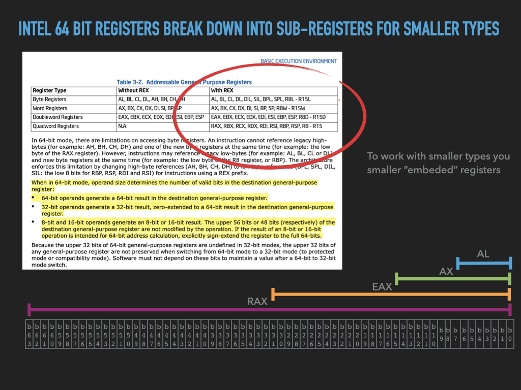
On modern processors like 64 bit Intel and ARM processors, the GPRS are all 64 bits (8 bytes) in length. However, the processors also provide GPRS of smaller lengths which refer to subcomponents of the 64bit registters. For example, on 64 bit ARM processors, the names W0..W30 refer to 32 bit (4-byte) length registers which are formed from the lower 32 bits of the corresponding 64 bit X register. Intel Processors have a much more diverse and subtle set of smaller sized registers that are composed of the sub-bytes of the 64 bit GPRS. The figure below illustrates an example of the Intel names for smaller registers that refer to bytes of a larger register.

Fig: Example of how the INTEL GPRS are broken down. Note one must carefully read the manual as the breakdown is not the same for all the GPRS.

17.2.1.1. Notation

When we want to name a register location we will extend our notation as follows. If we are referring to a particular processor vendor register, we will use the name subscripted with the length to avoid confusion. For example, to note that we are assigning the value in the Intel 64 bit RAX register to RBX we would write \(\text{RBX}_{64} \leftarrow \text{RAX}_{64}\). Similarly, in the case of ARM we would write \(\text{X2}_{64} \leftarrow \text{X1}_{64}\). If we are generically referring to registers we will use capital scripts notation subscripted by a specific length as follows \(R4_{32} \leftarrow R5_{32}\).

17.2.1.2. GDB Display and Set Registers

GDB: The following are some basic gdb commands for working with registers. We will learn more advanced syntax later but this will get us going.

• p /t $<register name> : print out the current value of a register in binary notation

• set $<register name>=0b<binary value : to set a register’s value in binary notation

• p /x $<register name> : print out the current value of a register in hex

• set $<register name>=0x<hex value> : to set a register’s value in hex notation

As we see in Intel Register Figure. Each register name references an exact size in bytes. Eg. rax is a 64 bit (8-byte) register so setting its value is an 8-byte assignment vs eax is 32 bits (4 bytes) in size, being a 4-byte assignment. GDB will add leading zeros as necessary to pad out any value that is smaller than the size of the register. Similarly, gdb will ignore all lead values that are beyond the size of the register.

The gdb command p stands for print. GDB has many built in encodings and notations that it understands. In the above, the /t and /x specified the format, or notation, we wanted to print the value in. More generally, the format syntax is very rich. The print command format syntax is a restricted set of the examine memory command (x) format syntax. We will discuss examining memory when we discuss working with memory in GDB later in this chapter. Remember, you can use the help command in gdb to learn more about any command. However, the help documentation can be a little overwhelming at first.

Open the following to see an x86-64 example session using these commands (we encourage you to try this yourself and to play around).

1. assemble and link the empty256.s code shown

2. gdb: Start gdb

3. file empty256: Open the empty256 executable

4. b _start: Set a breakpoint at _start

5. run: Start/run "inferior process" from executable

6. When execution stops at breakpoint 6 p /t $rax: print register rax in binary

7. set $rax=0b10101111: set register rax to 10101111 in binary (leading zeros are added automatically)

8. p /t $rax: print rax again in binary

9. p /x $rax: print rax in hex

10. set $rax=0xfeedface: set register rax

11. set $rbx=0xdeadbeef: set register rbx

12. p /x {$rax, $rbx} : print both registers in hex

13. p /t {$rax, $rbx} : print both registers in binary

14. set $cl=0xcafe set byte sized cl register with a two-byte sized value

15. p /x $cl : print byte register in hex

16. p /x $cx : print two-byte register in hex

17. p /x $ecx : print three-byte register in hex

18. p /x $rcx : print eight-byte register in hex

CODE: Source to create an empty process with 256 bytes of zeros to play with in gdb

	.intel_syntax noprefix        # syntax directive
	.text                         # linker section <directive>

	.global _start                # export symbol _start to linker
_start:                           # start symbol
	.fill 256, 1, 0x00            # https://sourceware.org/binutils/docs/as/Fill.html

Commands to assemble and link

GDB Session

17.2.2. Memory, addresses and address expressions

In a von Neumann architecture, the Memory of the computer forms a large, fixed-size array of bytes which is directly connected to the CPU. Critically, the CPU can transfer values from and to its registers and locations in memory. Unlike registers, there are no hardware-specific symbolic names for these locations. Rather, we identify which byte of memory by specifying its array index, which we call its address.

17.2.2.1. Notation

We will use \(M[\text{<expr>}]\) to refer to a specific byte in memory, where \(\text{<expr>}\) is an address expression whose value is the address we are referring too. In the simplest from, this might just be a number in some base notation eg. \(M[\text{0xFFF0}]\) refers to the memory location of the byte at address \(\text{0xFFF0}\). We might also use symbols such as \(\alpha\) or \(\beta\), to mean some particular address but whose exact value is not of concern eg. \(M[\alpha]\). It is important to note that an address is just a number ranging from 0 to the maximum number of bytes of memory minus one. This range is often called an address space, as it defines the range of memory addresses that one can refer too. On a computer that supports a \(2^{64}\) address space, the address values can range from \(0\) to \(2^{64}-1\) or in hex \(\text{0x0}\) to \(\text{0xffffffffffffffff}\).

Given that an address is just a number, it is natural for an address expression to be a simple arithmetic expression eg. \(M[\alpha + 16]\) means the memory location whose address is \(\alpha\) plus 16. Similarly \(M[\beta + 8 * \alpha]\) means the memory location whose address is \(\beta\) plus eight times \(\alpha\). It will also be common for us to use the value of registers in memory address expressions, such as \(M[\text{RAX}_{64} + 4 * \text{RDI}_{64} + \text{0xdeadbeef}]\) which means the location which is the current value of \(\text{RAX}\) plus 4 times the current value of \(\text{RDI}\).

Finally, we may want to work with a group of bytes of a length \(w\) (in bits) starting at a particular address. Like with registers, we will use a subscript to indicate the length eg. \(M[\alpha]_{16}\) or \(M[\alpha]_{32}\) or \(M[\alpha]_{64}\) respectively meaning the 2, 4 and 8 bytes starting at location \(\alpha\) and proceeding the the next larger locations as needed. If no length is given, then we implicitly mean a length of 8 bits (1 byte).

As before, we will use the \(\leftarrow\) to indicate assignment: eg.

• \(M[\text{0xdeadbeef}] \leftarrow \text{0x1a}\) means set the bits of the byte at memory address \(\text{0xdeadbeef}\) to the value of \(\text{0x1a}\).

• \(M[\alpha + 8 * R13_{64}]_{64} \leftarrow R5_{64}\) means set the bits of the 8 bytes at the memory address who’s value is \(\alpha\) plus eight times the 8 bytes value of register \(R13\) to the 8-byte value of register \(R5\).

• \(\text{RAX}_{64} \leftarrow M[\text{RIP}_{64} + -42]_{64}\) means set the 64 bit value of the \(\text{RAX}\) register to 64 bit value at memory whose address is the current 64 bit value of the \(\text{RIP}\) register minus 42.

17.2.2.2. Byte Geometry

Given that we have settled on the byte as the standard unit of storage, we unsurprisingly measure capacity of devices in bytes. For example, my computer has 32 GigaBytes of memory and a 1 TeraByte Solid State Drive. Similarly, when we encode information, the encoded information has a length in bytes. As a matter of fact, one can go further to say that information has a geometry in the form of a position (location) and size (length in bytes).

We will find that it can be very useful to learn how to visualize the geometry of our software, both to understand how it is being represented, and how and why it works the way it does.

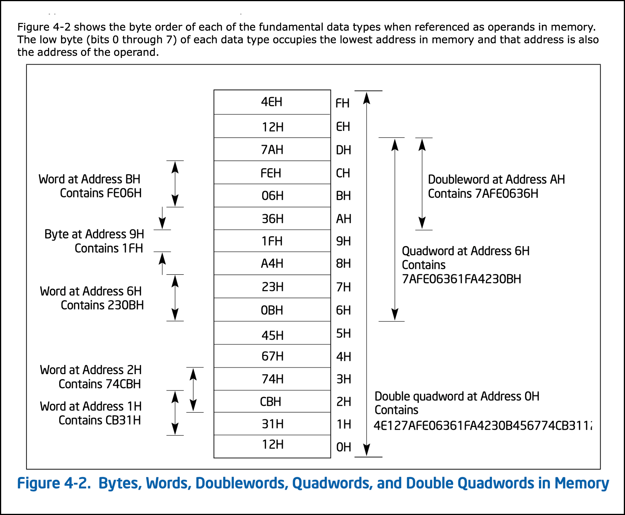
17.2.2.3. Multi-byte quantities

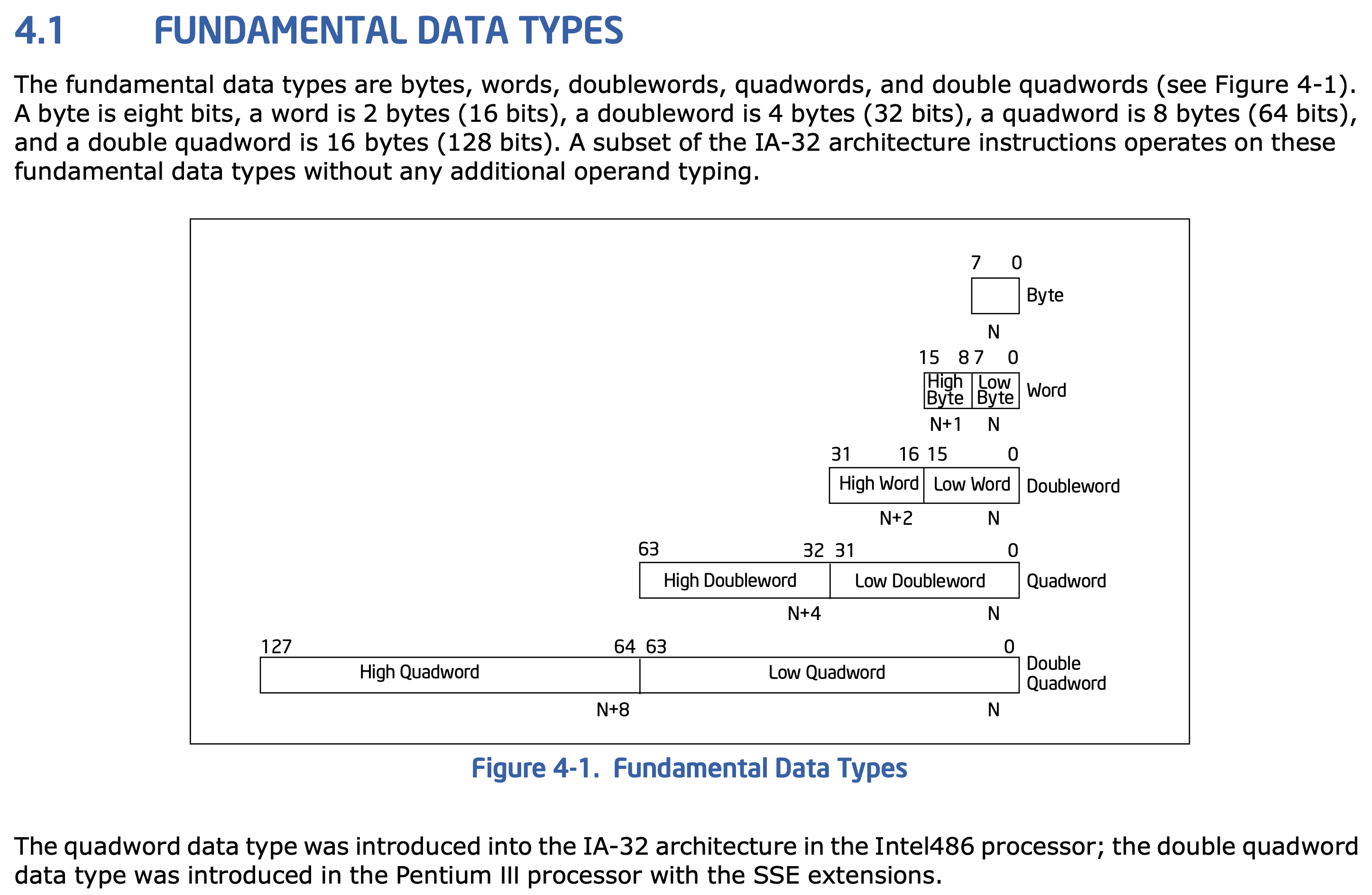
As we saw above, CPUs have evolved to contain GPRS that are bigger than a single byte. Given this, they typically integrate instructions that work with a fixed set of multi-byte values. Most processors today directly support operations on one, two, four and 8-byte values.

As an example, the following figure is an extract from the INTEL software development manuals explaining the support their CPUs have for working with 1,2,4,8 and 16-byte quantities. In our coverage, we will not look at sizes greater than 64 bit as these tend to be custom and not uniformly supported across processors.

Figure: Extract from INTEL Software Development Manuals discussing the multi-byte quantities that it has built in support for working with. This means these values of these sizes can be moved in and out of the processor and that the processor contains operations that can work on them.

Many processors today integrate custom support for even larger multi-byte values such as 128, 256 and even 512 bits. Such larger quantities, and the registers that support them, are often used for a mode of operation called vector processing. In this mode, the large group of bytes are used to hold a vector of values that are operated on as a group. For example, one might use such registers to hold a vector of 128 four-byte quantities that can be operated on together. One such operation could be to add one vector of values to another vector of values using a single instruction. Internally, the processor has support for doing independent calculations concurrently. This is actually a model of parallel processing called Single Instruction Multiple Data (SIMD). SIMD operation is critical to achieving high performance when working on data intensive applications. This includes linear algebra intensive Machine Learning/AI and graphics applications. Examples of such support are INTEL’s AVX512 and ARM’s SVE. A hallmark of Graphics Processing Units (GPUs), and their usefulness for improving the performance of Machine Learning tasks, is their support for vector processing and SIMD operation.

17.2.2.4. “Endianness”

Given support for multi-byte values, a decision needed to be made regarding the order that is used to store the bytes of a multi-byte register when it is transferred to or from memory.

For example if we want to do the following: \(M[\alpha]_{64} \leftarrow R1_{64}\)

We must transfer the 64 bits (8 bytes) of \(R1\) to memory starting at address \(\alpha\). The first choice that was made was to store the bytes of the register in increasing address order. That is to say the bytes of the Register will be stored at the bytes in memory whose addresses are increasing. So in our example, the 8 bytes of \(R1\) will stored at: \(M[\alpha]_{8}\), \(M[\alpha+1]_{8}\), \(M[\alpha+2]_{8}\), \(M[\alpha+3]_{8}\), \(M[\alpha+4]_{8}\), \(M[\alpha+5]_{8}\), \(M[\alpha+6]_{8}\), and \(M[\alpha+7]_{8}\). While there are many possible order that could be used two standard “endiannesses” that developed; 1) little endian, and 2) big endian.

Before we can present the two standard orders, we must first have a convention for referring the the bytes of multi-byte value. We use the mathematical notion of significance.

17.2.2.4.1. Most and Least Significant Bytes

Figure: Byte Significance

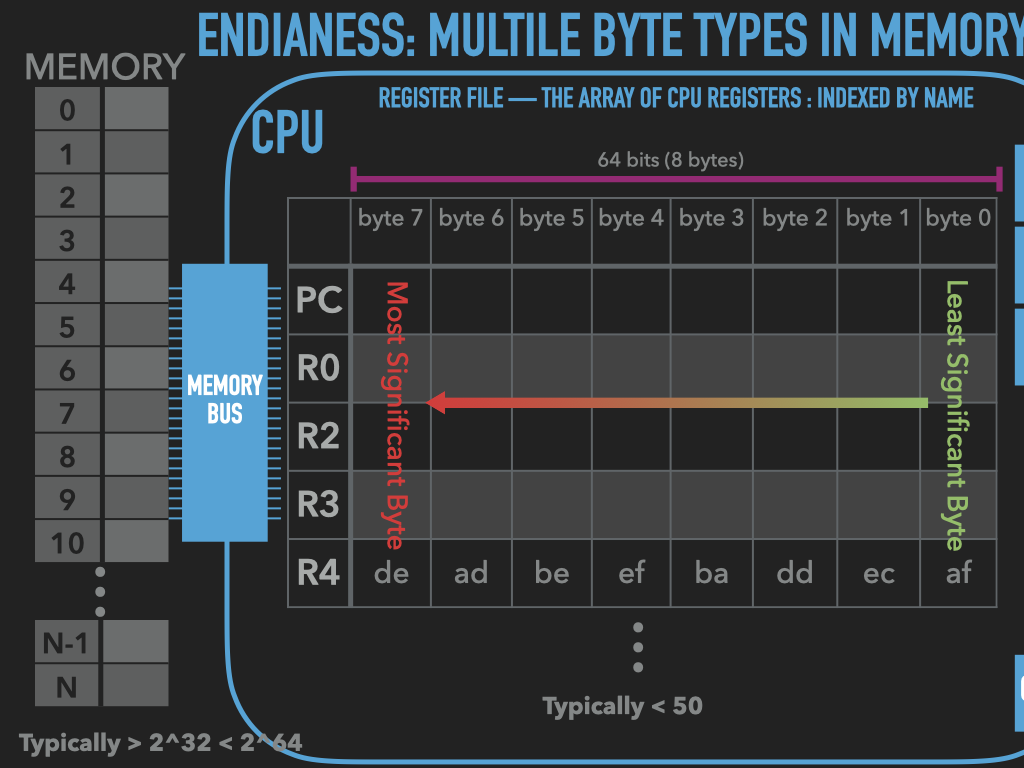
Given that we think of a binary value as a vector of bits, it is natural to think of them as a vector of bytes with the same notion of significance of bits. As illustrated above.

17.2.2.4.2. Little Endian

Figure: 'Little Endian' byte ordering.

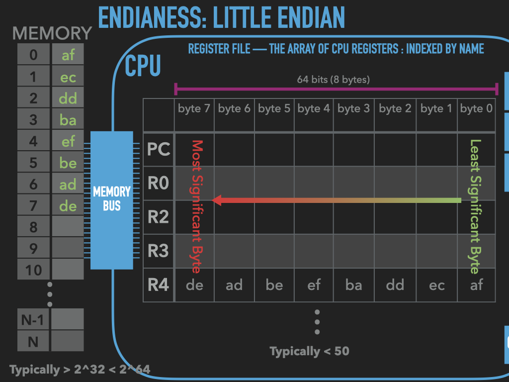
Little Endian byte ordering places the bytes in memory from least significant to most as illustrated in the figure above.

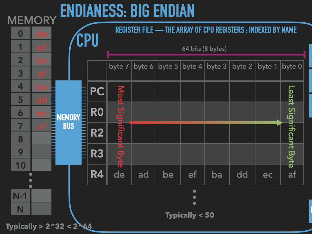
17.2.2.4.3. Big Endian

Unsurprisingly Big Endian byte ordering places values from most significant to least, the direct opposite of little endian ordering.

Figure: 'Big Endian' byte ordering.

17.2.2.4.4. Why Endianness matters to us

The CPU (and computer more generally) is configured to operate either in Little Endian or Big Endian byte ordering. For most programmers this detail is hidden from them. But for those of us who want to look under the covers, we need to be aware of which ordering the hardware is configured to use. When we look at the raw bytes in memory and want to interpret a group of them as a single vector, in the same way that the CPU will, then we must know the ordering. As we can see in the prior figures, if we where to assume wrong ordering our interpretation of the value would be very different that the CPU’s.

It is also worth realizing that when we want to exchange raw binary information between computers we will also have to account for endianess. This includes files that contain binary data that we want to work with on two different computers and binary data we exchange on the internet. Programmers over the years have carefully chosen what order to use, and developed functions to convert the ordering of the data to the ordering used by the computer that is accessing the data. The wikipedia page on Endianness discusses both the implications on files and networking

Figure: Extract from the INTEL Software Development manual discussing byte ordering of multi-byte values in memory. Note INTEL use a sufix of 'H' to denote that a value is expressed in hex notation.

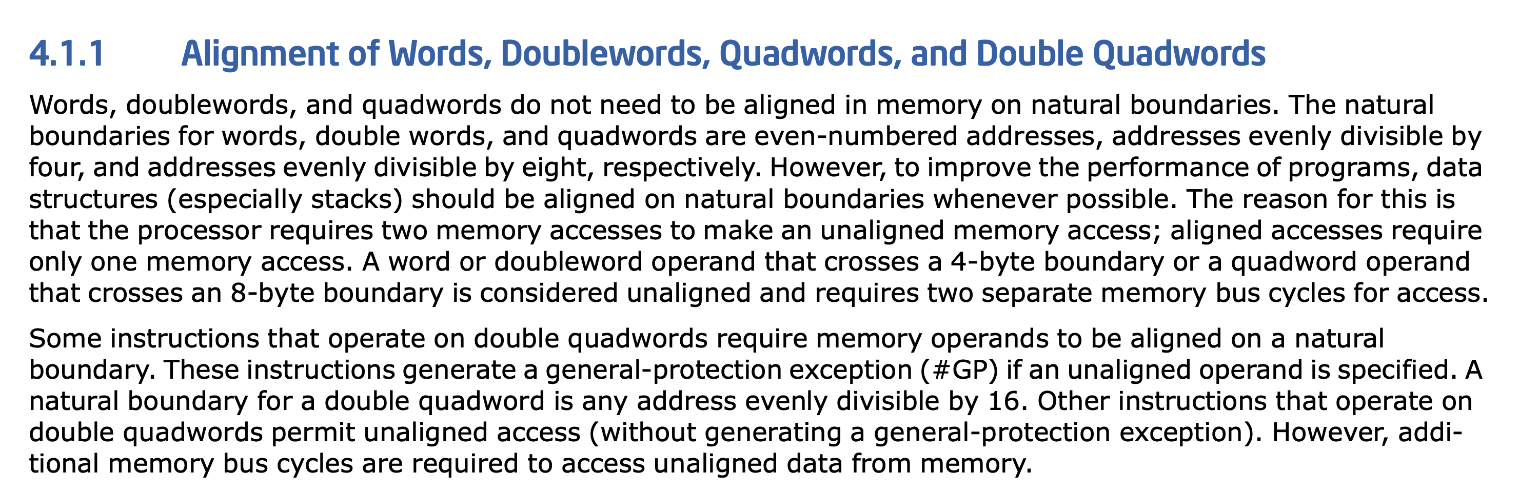
17.2.2.5. Alignment

Like endianness there is another detail, called alignment, that we will run into when looking at and placing values in memory. Modern CPUs and operating systems may place restrictions on the addresses that we can place values of particular sizes at. In some cases, these restrictions are strict, and violating them will trigger an error that the operating system will have to take care of, potentially causing it to terminate our program. In other cases, not adhering to the restrictions will only reduce the performance of our program.

Alignment restrictions are typically specified in the following form: \(w\) byte values must be \(a\)-byte aligned. Which means that the address that we place a value that is \(w\) bytes in length must be divisible by \(a\). For example, a common alignment we will run into is that four-byte quantities must be four byte aligned. This means that that the addresses at which we place four-byte values in memory must be divisible by four. In binary notation, the addresses that satisfy this alignment are those whose two least significant bits are zero. The figure below is an example discussion of memory alignment from the INTEL software development manuals”.

Figure: Extract from INTEL Software Development Manuals discussing memory alignment.Note: In INTEL terminology words, double words and quadwords are 2-byte (16 bit), 4-byte (32 bit) and 8-byte (64 bit) quantities.

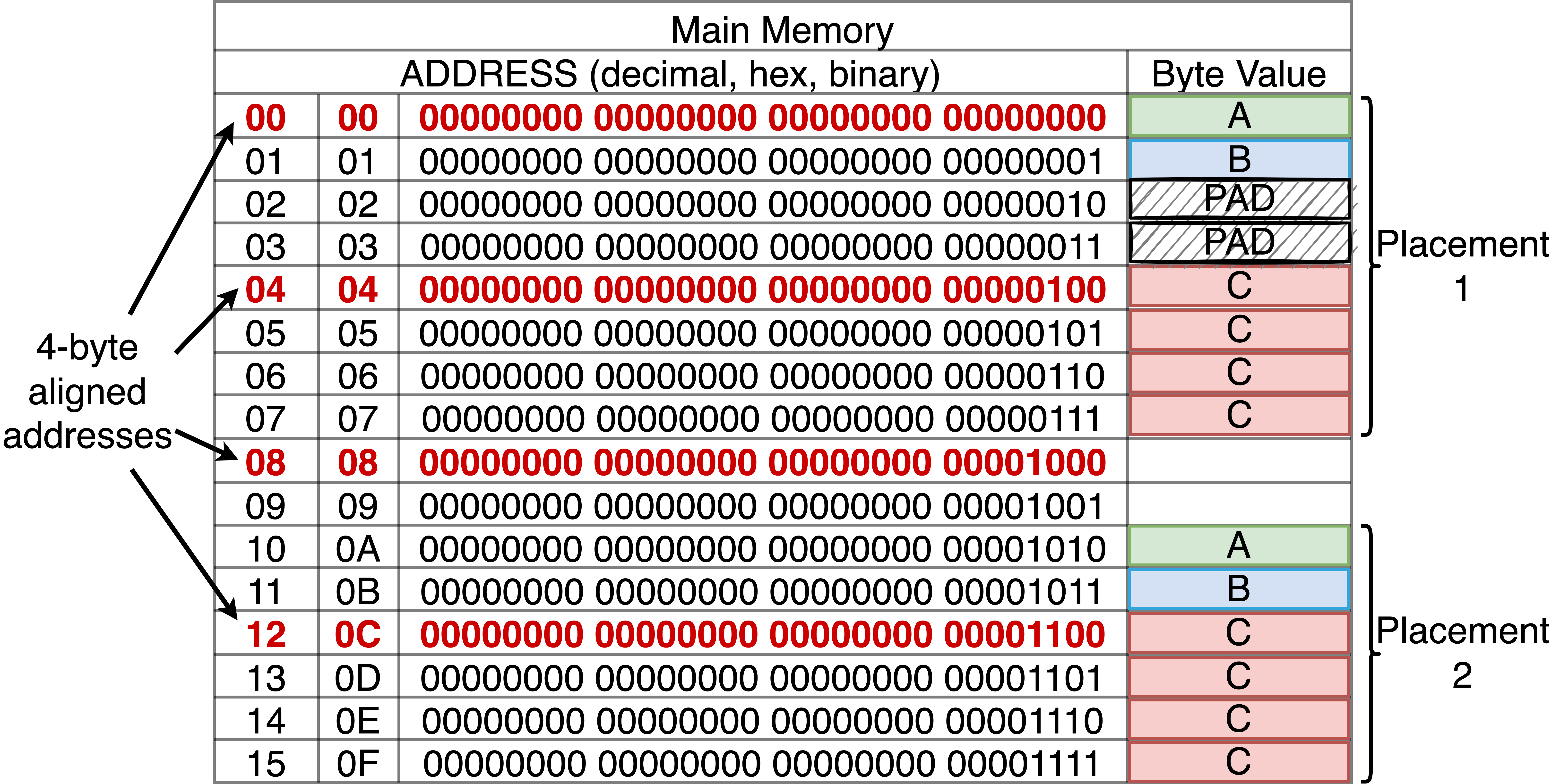
Practically, this means that when we are exploring memory, or laying things out in memory, we might need to account for alignment. In particular, we will run into the use of “padding” bytes in order to ensure correct alignment can be achieved. For example, lets assume that we want to place two one-byte values, \(A_8\), and \(B_8\) followed by a four-byte value \(C_{32}\) consecutively in memory. A and B as single-byte values do not have any alignment restrictions and can be placed any where in memory. However, we will assume that the four-byte value C must be 4-byte aligned. The figure below illustrates two placements, 1 and 2, of these three values in the first 16 bytes of memory (main memory locations with addresses in the range of 0-15).

Figure: This figure illustrates how alignment requirements can affect how things get laid out in memory. See the text for a dicussion.

On the left of the figure are the addresses of each memory location in decimal, hex and binary notation. The addresses in red are those that satisfy 4-byte alignment, exact multiples of 4. Note in binary this corresponds to the locations that have zeros in their two least significant bits. The right side illustrates locations that can store a byte value associated with each address. The values A, B and C are illustrated as byte-sized boxes shaded green, blue and red respectively. Given that C is four bytes, it requires 4 consecutive memory locations. Two possible placements, 1 and 2, for the three values are shown. Again, we assume it is a requirement to place the values in the specified order and consecutively in memory.

In placement 1 A is placed at address 0. Given that B is one byte, there is no restriction on where it can be placed and as such, it can be directly placed at address 1 next to A. C however requires 4-byte alignment and thus cannot be placed at address 2 or 3, so we must skip these bytes and the first location that C can be placed is 4. We call the bytes at 2 and 3 padding, as they are unused bytes only consumed to ensure alignment requirements.

Placement 2 starts placing the three values at address 10. Again, given that A and B have no restrictions on where they can go, they are assigned to addresses 10 and 11. Given these placements, the next address is 12 - which is four-byte aligned - so C can placed here with no need for padding.

Notice in the first 16 bytes there are exactly four locations that we are allowed to place C, and as such there are only three possible placements for our data. The other placement that can be used would place A and B at addresses 6 and 7 so that C aligns to address 8. Without alignment constraints, we could have placed the data beginning at any address from 0 - 10 and not required padding bytes for any of them.

When programming at the level of directly controlling memory we can see that there are various impact the choices we make can have. Notice different placements can result in the need to waste bytes on padding while others do not. Similarly the order that we choose for our data can affect our placement as well. In the example had we ordered A and B after C then we could have placed the data at address zero without requiring padding. Similarly had we ordered C in between A and B then we would have required three pad bytes to place the at address zero! It is worth noting that when we use higher level programming languages and tools the decisions and constraints still exist but must be made and met by the languages and tools.

17.2.2.6. GDB and Memory

GDB: GDB have very rich support for working with memory. We can refer to addresses and various ways, examine memory at an address in many sizes and formats, and we can also set the value at memory locations. It will take time for us to learn all this syntax. But lets start with some basics commands to display addresses and examine the values starting at an address.

1. p &<symbol> will print the address of a name that we have used in our program that gets assigned an address by the linker. Eg. “_start”

2. x /1bt <address> will print one byte in binary starting at the address specified

3. x /1bx <address> will print one byte in hex starting at the address specified

4. In 2 and 3 above you can replace the b with h or w or g. This sets the size of unit to print b sets the unit size to 1 byte, h - 2 bytes, w - 4 bytes and g - 8 bytes. Eg. x /1gx will print an one 8-byte value (unit) starting at the specified address. GDB will take care of endianness for us.

5. In 2 and 3 above you can replace 1 (the number of units) with an integer \(n\) to display \(n\) units.

As we discuss more representations we will be introduce more complex formats for examining values.

To set the value of a set of bytes starting at and address is a little more complicated as gdb uses syntax from the C programming language. Given that we have not yet covered the C programming language we will start slowly and introduce what we need as we go. To start with lets see how we set 1, 2, 4 and 8-byte vectors starting at an address to hex and binary. Like registers we use the set command but it is our job to tell gdb using a C type what size we are working with. Respectively the types we will use are unsigned char, unsigned short, unsigned int and unsigned long long. The following summarizes the syntax we will use for the moment:

1. set {unsigned char}<address>=0x<hex value> to set a single-byte value starting at the specified address to the given value.

2. set {unsigned short}<address=0x<hex value> to set a two-byte value starting at the specified address to the given value.

3. set {unsigned int}<address=0x<hex value> to set a four-byte value starting at the specified address to the given value.

4. set {unsigned long long}<address=0x<hex value> to set a eight-byte value starting at the specified address to the given value.

Like when setting registers gdb will add leading zeros or truncate the the right most digits if the size we specify is larger or smaller than the value we provide. The following example gdb session illustrates using this syntax.

1. assemble and link the empty256.s code shown

2. gdb: Start gdb

3. file empty256: Open the empty256 executable

4. b _start: Set a breakpoint at _start

5. run: Start/run "inferior process" from executable

6. When execution stops at breakpoint 6 p &_start : print the address of where _start was put into memory.

7. x /1bt &_start: examine 1 byte in binary at the address of _start in binary

8. set {unsigned char}&_start = 0b10101010 : set the byte at the address of _start

9. x /1bt &_start: examine the 1 byte at the address of _start in binary again

10. x /1ht &_start: examine the 2-byte value at the address of _start

11. x /1wt &_start: examine the 4-byte value at the address of _start

12. x /1gt &_start: examine the 8-byte value at the address of _start

13. x /1bx &_start: examine the 1 byte at the address of _start in binary again

14. x /1hx &_start: examine the 2-byte value at the address of _start

15. x /1wx &_start: examine the 4-byte value at the address of _start

16. x /1gx &_start: examine the 8-byte value at the address of _start

17. x /8bx &_start: examine 8 bytes as single byte values at _start

CODE: Source to create an empty process with 256 bytes of zeros to play with in gdb

	.intel_syntax noprefix        # syntax directive
	.text                         # linker section <directive>

	.global _start                # export symbol _start to linker
_start:                           # start symbol
	.fill 256, 1, 0x00            # https://sourceware.org/binutils/docs/as/Fill.html

Commands to assemble and link

GDB Session

17.2.2.7. Fixed widths and their implications

It is very important to realize that when we refer to a register or memory location we must always keep in mind the length of the location. As we saw each register has a fixed length specified by the CPU maker. Eg. The INTEL registers \(RAX\), \(EAX\), \(AX\), \(AL\) are \(64\), \(32\), \(16\) and \(8\) bits long respectively and the ARM registers, \(X0\) and \(W0\) are \(64\) and \(32\) respectively. When dealing with memory it our responsibility to explicitly transfer the right length in bits (to or from memory). For example generically, on modern 64 bit cpus, given an address \(\alpha\) and a 64 bit GPR such as \(R3_{64}\) the following transfers are all typically possible.

1. \(R3_{64}\) \(\leftarrow\) \(M[\alpha]_{8}\), \(M[\alpha]_{8}\) \(\leftarrow\) \(R3_{64}\)

2. \(R3_{64}\) \(\leftarrow\) \(M[\alpha]_{16}\), \(M[\alpha]_{16}\) \(\leftarrow\) \(R3_{64}\)

3. \(R3_{64}\) \(\leftarrow\) \(M[\alpha]_{32}\), \(M[\alpha]_{32}\) \(\leftarrow\) \(R3_{64}\)

4. \(R3_{64}\) \(\leftarrow\) \(M[\alpha]_{64}\), \(M[\alpha]_{64}\) \(\leftarrow\) \(R3_{64}\)

There will be separate instructions for each. As such it will always be our responsibility to specify the length of the transfer in addition to the direction and address! When the sizes of a transfer do not match we must also be aware of what will happen.

17.2.2.7.1. Truncation

Most CPUs when transferring a larger vector to a smaller vector eg. \(R3_{8}\) \(\leftarrow\) \(R4_{32}\) or \(R2_{16}\) \(\leftarrow\) \(M[\beta]_{64}\) the most significant bits of the value will be truncated to fit. For example if we were transferring the following \(32\) bit value:

b31	b30	b29	b28	b27	b26	b25	b24	b23	b22	b21	b20	b19	b18	b17	b16	b15	b14	b13	b12	b11	b10	b9	b8	b7	b6	b5	b4	b3	b2	b1	b0
1	1	1	1	1	1	1	1	1	1	1	1	1	1	1	1	1	1	1	1	1	1	1	1	0	0	0	0	0	0	1	1

When transferring to an 8 bit location we would end up with bits \(8\) to \(31\) being truncated leaving us the following value in destination.

[b7	b6	b5	b4	b3	b2	b1	b0]
0	0	0	0	0	0	1	1

17.2.2.7.2. Trunction and Modulus

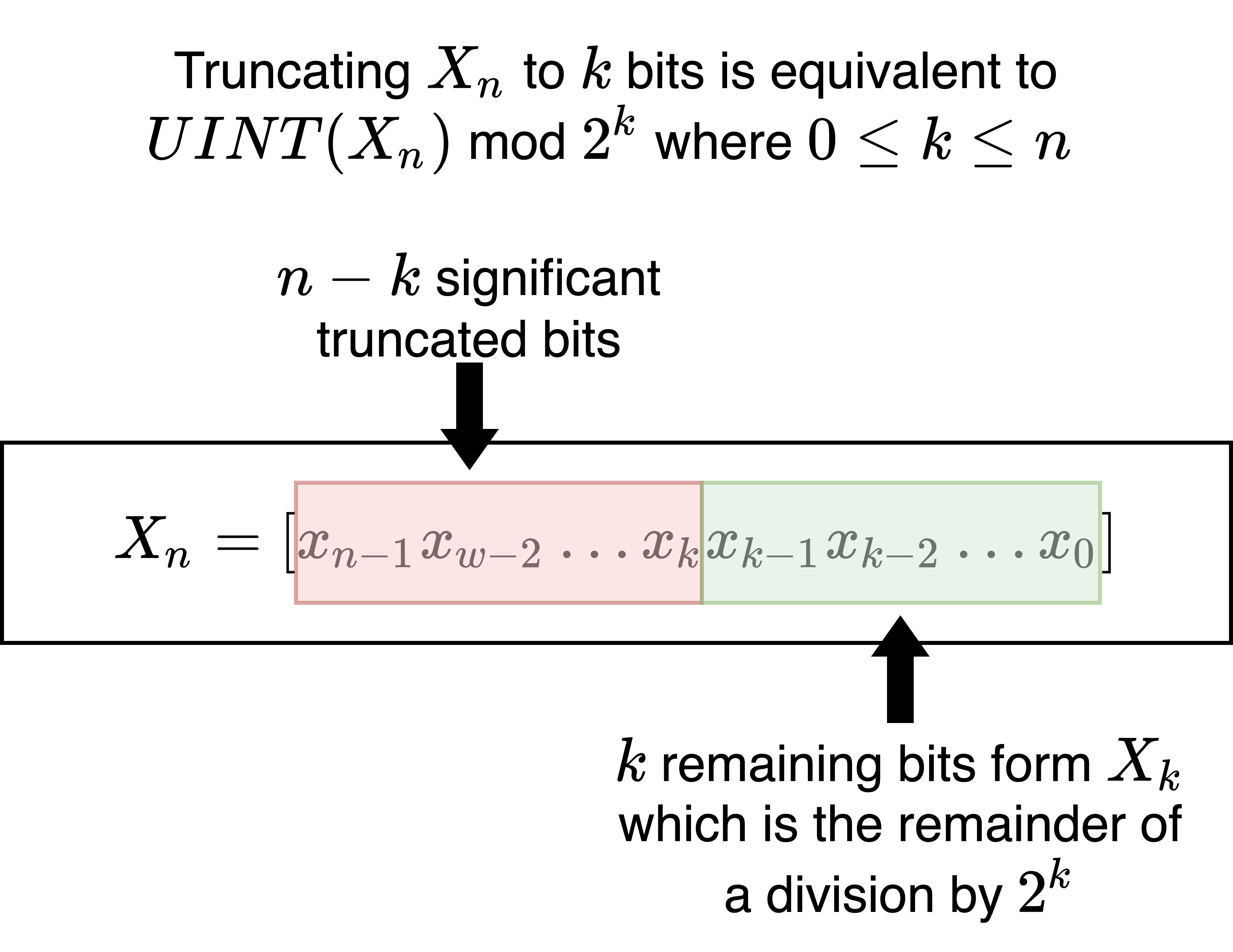
More generally when we truncate an \(n\) bit value \(X_{n}\) to its least significant \(k\) bits (\(k \leq n\)) \(X_k\) we loose the most significant \(n-k\) bits. When interpreting the values as unsigned integers, truncation is equivalent to

\[UINT(X_k) = UINT(X_n) \text{ mod } 2^k\]

Figure: Trunction and Modulus

The “fixed” width in bits of locations will often lead to us having to deal with the limit it imposes. These limits lead to unfortunate problems, such as overflow and underflow, when using bytes to representing and work with numbers. We will discuss these problems in more detail later.

17.2.2.7.3. Extension

When transferring values from smaller locations to larger locations we must decide how to expand the value.
For example to moving a 32 bit located in memory at \(\alpha\) into a 64 bit register, \(R5_{64} \leftarrow M[\alpha]_{32}\). CPUs typically support various operations that let us dictate how the unspecified bits of the destination should be set.

The two most common strategies that we will encounter are zero and sign extension. The former simply means extending the source smaller value with leading zero bits to create the larger value. Signed extension is more subtle and we will deffer its discussion to when we discuss how we represent signed integers as binary vectors.

A third option that one might also encounter is to leave the bits of destination, that the smaller value does not provide values for, unchanged.

17.3. Representing Text (Opcodes) and Data

When discussing the von Neumann architecture we introduced the two broad, and not necessarily mutually exclusive, categories of information we want to represent: Text and Data (opcodes). So now that we know that registers and memory are arrays of bits our job is to understand how we can use binary to represent and work with Text and Data.

17.3.1. Text

As we discussed, in the introduction to this part of the book, the CPU provides us with a binary code called machine code that we can use to encode the operations of our program. In von Neumann architecture chapter saw that the CPU has a built in Execute Loop that fetches, decodes and executes encode instructions that we load into memory. We also read in the introduction that the task of programming in machine code is simplified by a tool called an assembler. The assembler lets us write our programs in Assembly Language. The assembler has built into it the CPU’s encoding.
This allows us to write ASCII mnemonics, English short hands, that the CPU manual documents, into a file. By running the assembler with our file as input it will translate our assembly code into the binary equivalent that encodes the operations.

Given that we have assemblers our main job as programmers is not to memorize the binary code. Rather our task is to learn what the operations of a CPU can do and how to use and structure them properly to create out programs using the an assembler and linker. As we read the operations roughly break down into three categories:

1. Perform Arithmetic and Logic (eg. adding and comparing numbers)

2. Transfer bytes into and out of the CPU

3. Control what happens next by controlling how the PC gets updated.

How we combine theses operations and lay them out in memory to create standard programming structures, like “if statements”, “loops”, “functions” and complex data structures are the topics of the “Program Anatomy” chapters.

GDB: One the most powerful aspects of gdb is its built in support for the cpu machine code encoding. Specifically, it has the support for “disassembling” location of memory. That is to say it can decode the opcodes in memory and print to its user the mnemonics that they correspond too. As mentioned before the examine memory command x support several format specifiers. One of them is i which means that that the memory location being examined should be decoded as an instruction. GDB will examine the location and use its built in disassembler to translates the bytes at that location into the CPU mnemonic it corresponds to. CPU’s like INTEL can use several bytes to encode a single instruction and as part of disassembly GDB will know where this instruction ends. If a count is given to the examine command along with the i format gdb will go on and attempt to disassemble successive memory addresses necessary to print the number of instruction specified. The following shows and example of this using a simple assemble program. You don’t need to worry to much about what this programming is doing at this point main thing to note is gdb’s ability to reverse the process of the assembler. Note in the below example we do not need to create a process to disassemble it as the memory values can all be read directly form the binary executable file.

1. assemble and link the oneplusone.s code shown

2. gdb: Start gdb

3. file oneplusone: Open the oneplusone executable

4. set assembly-flavor intel: switch to intel syntax for disassembly output

5. x/1i &_start: examine the memory starting at the address of _start as 1 instruction

6. x/4i &_start: examine the memory starting at the address of _start as 4 instruction

Note:

1. We do not need to start the program as the text can be directly read from the executable

2. How gdb automatically moves forward the right number of bytes when decoding

CODE: simple one plus one program to test out gdb disassembler

	.intel_syntax noprefix        

	.text                         
	                              	                         
	.global _start     
_start:                    
	mov al, 1        # transfer 1 into al
	add al, 1        # add 1 to the value in al
	nop              # do nothing -- requires only one byte to encode
	mov bl, al       # transfer value in al to bl
	

Commands to assemble and link

GDB Session

17.3.2. Data

Given that all value in the computer are really just collections of bytes we must represent all the data of our programs in binary. Over the years we have developed many encoding like ASCII that we use to represent and work with our data. The encoding provide us when standard interpretations for both representing things as bytes and working on them. The encoding roughly break down into two big categories:

1. Native Types: The CPU provides operations that understand the encoding and provides functions that works with encoded values. While different CPUs support various specialized encodings there are four that all modern CPUs support:

   1. Raw bit and byte boolean oriented functions

   2. Unsigned integers

   3. Signed integers

   4. Floating point numbers

2. Software supported: These are the more complex encodings that we create by writing software using the built in encodings of the CPU. We categories these into two:

   1. Programmer Defined Types: Building on the capabilities of the hardware we introduce our own data types that use the native types, memory, and functions we write to provide to make composing our programs easier. Examples include Arrays, Structures, Stacks, Linked Lists, Trees, Objects, etc. Many high level programming languages provide direct support for these. However, they are generally not native to the hardware and the authors of the programming language provided code to create them. When programming in assembly code we must use the native operations and memory organizations to create them.

   2. Standardized Data Formats: We know many of these as “file types”. Examples include: “pdf”, “jpeg”, “png”, “mp4”, “html”, “elf”, etc. Others exist as protocols that we use to exchange data on networks. Examples are “Ethernet”, “IP”, “UDP”, “TCP/IP”, etc. Standardized data formats are generally defined by standardization bodies that publish documentation that tell programmers exactly how the data is represented and what standard operation need to be supported. More often than not libraries of software are provided that allow you to work with these data encoded in these formats without having to write implement the operations.

Our focus will be to understand the Native Types and Programmer Defined Types. The later we will discuss part of our coverage of program anatomy. With an understanding of these you can go on to but understand the Standardized Data Formats and for that matter create your own.

GDB: Gdb has built-in support to help us encode and decode the native types of the hardware. Using this support can be very useful in learning how these types are represented in binary. To do this we must know how to tell gdb what types we are working with. As mentioned before the print and examine command support several data formats that correspond to the native types of the cpu. See help examine output in the example below. In order to set a value to a specific type we must carefully specify the value in a way gdb knows what encoding to use. We will look at these in more detail as we examine the various encodings. Note the assemble also understands various encodings to make our job easier when writing assembly code as well. In the following we will only use the examine syntax and the ability to enclose a ASCII character in single quotes to tell gdb to encode it into a binary value. Another things we illustrate is gdb’s knowledge of the fact that ASCII strings are by convention encoded as a sequence of memory locations encoded in ASCII terminated by a location that has the value zero.

1. assemble and link the empty256.s code shown

2. gdb: Start gdb

3. file empty256: Open the empty256 executable

4. b _start: Set a breakpoint at _start

5. run: Start/run "inferior process" from executable

6. help x

7. When execution stops at breakpoint

8. set $al = 'h': use ASCII encoding to set al to the byte value of 'h' in ASCII

9. p /x $al: print value of al in hex

10. p /t $al: print value of al in binary

11. p /u $al: print value of al as an unsigned integer

12. p /d $al: print value of al as a signed integer

13. p /c $al: print value of al as a ASCII character

14. set $al = 0xff : set al to hex 0xff

15. p /x $al: print al in hex

16. p /t $al: print al in binary

17. p /u $al: print al as an unsigned integer

18. p /d $al: print al as a signed integeter -- surprised?

19. set {unsigned char}(&_start) = 'h': set byte at address of _start to value of ASCII h 19 set {unsigned char}(&_start+1) = 'e': set byte at address of _start + 1 to value of ASCII e

20. set {unsigned char}(&_start+2) = 'l': set byte at address of _start + 2 to value of ASCII l

21. set {unsigned char}(&_start+3) = 'l': set byte at address of _start + 3 to value of ASCII l

22. set {unsigned char}(&_start+4) = 'o': set byte at address of _start + 4 to value of ASCII o

23. set {unsigned char}(&_start+5) = 0x00: set byte at address of _start + 5 to 0

24. x /s &_start: standard way to encode an ASCII string is as a sequence of ASCII values terminated by a zero

CODE: Source to create an empty process with 256 bytes of zeros to play with in gdb

	.intel_syntax noprefix        # syntax directive
	.text                         # linker section <directive>

	.global _start                # export symbol _start to linker
_start:                           # start symbol
	.fill 256, 1, 0x00            # https://sourceware.org/binutils/docs/as/Fill.html

Commands to assemble and link

GDB Session